DSMC and PICMC documentation

5.1.1 Geometric model

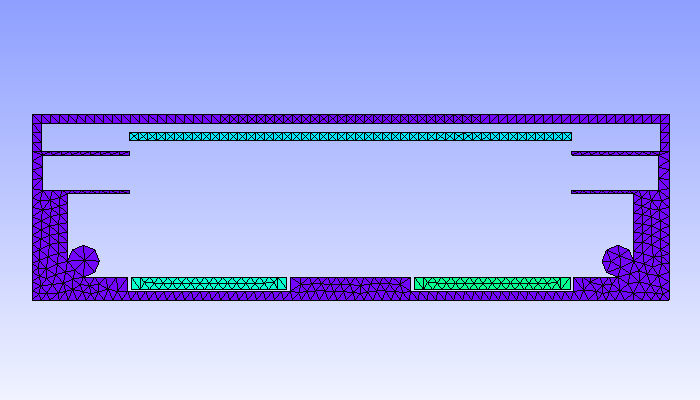
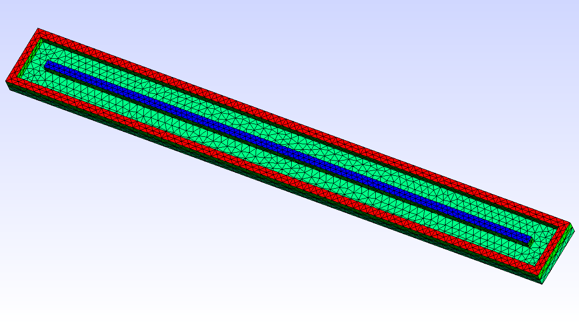
In this example, we simulate a plasma discharge in a dual-magnetron planar sputtering compartment in our Leybold-A700V sputter coater. The rectangular sputter targets are sized \(750\times 88\textrm{ mm}^2\) and are equipped with the unbalanced version of the PK750 magnet assembly (see Tab. 5.1).

For 2D plasma simulation, a 2D cross-sectional representation of the chamber geometry is used. The chamber geometry still should have a finite thickness in the third direction, which should be in the order of one cell spacing. In contrast, for the magnet, a 3D model is required. After solving the Laplace equation for the magnetic scalar potential on the magnet mesh, the magnetic field is computed in the 2D region of interest within the chamber model. Note: the actual magnet assembly can be located outside of the plasma simulation region, which is also the case in this example.

Table 5.1: 2D model of the sputter coater and 3D representation of the sputter target’s magnet assembly.

2D-model of a sputter compartment in the Leybold A700V coater	3D model of the unbalanced PK750 magnet assembly

The steps to create a complete simulation case out of the geometry files is described in the following.

5.1.2 Step 1: Unpack prepared files

Unzip A700V_PK750.zip into a directory, where the simulation case should be located. The ZIP file contains the GMSH files for the 2D chamber model and the 3D magnet model. The following files are included: * a700v.geo - GMSH model of the 2D chamber compartment * a700v.msh - The same model as *.msh file * pk750-single_standard_unbalanced.geo - 3D GMSH model of the magnet assembly * pk750-single_standard_unbalanced.msh - The same model as *.msh file

5.1.3 Step 2: Create and edit the parameter file

In a plasma simulation with magnetic field computation, two geometric models are required. The chamber geometry defines the region of interest, i.e. the region where the actual plasma simulation takes place. The magnet assembly can be located outside of the region of interest. A new parameter file always has to be generated from the meshed chamber model via the command

$ initpicmc a700v

Edit the a700v.par file in an ASCII editor of your choice. First we need to specify useful values for the time interval and time step for plasma simulation:

DT       = 5e-11;
TSIM     = 10e-6;

Set the workmode to plasma simulation:

WORKMODE = 1;

We have to adjust the power dissipation:

PSOLL = 10/750;

This corresponds to 10 W distributed over 750 mm target length. The 2D cross sectional model has a depth of 1 mm in the third direction, thus, the power has to be scaled by factor 1/750, where 750 mm corresponds to the real length of the sputter target in 3D.

Next step is to specify the list of species treated in the simulation. A minimal set for plasma simulation is a neutral gas molecule, its single charged positive ion and electron. For a plasma in Argon this includes the species Ar, Ar⁺, and e^-:

SPECIES = ["Ar", "Arplus", "e"];

The NREAL-parameter is the factor between the number of simulated and real particles and the P0-parameter is the pressure (for neutral particles like Ar) or the initial density (for charged Particles like Ar⁺ and e^-). The appropriate NREAL_Ar-parameter can be calculated from the total pressure and cell spacing (see below). Possible values for the other parameters are:

NREAL_Ar     = 5e9;
P0_Ar        = 0.5;
NREAL_Arplus = 1e5;
P0_Arplus    = 1e13;
NREAL_e      = 1e5;
P0_e         = 1e13;

Depending on what plots you are interested in during the simulation run, insert the species into the appropriate lists in the plotting section:

NUMBER   = ["Arplus", "e"];
DENSITY  = ["Arplus", "e"];
PRESSURE = ["Ar", "Arplus", "e"];
VELOCITY = ["Arplus", "e"];

The unit of the mesh geometry depends on the unit of the coordinates in the meshfile. In our example, the meshfile unit is 1 m, this the value of 1.0 for the UNIT variable is ok. The extent of the bounding box is calculated automatically from the a700v.msh-file, but we have to adjust the cell spacing. The bounding box has a volume of \(360\times 105\times 1\textrm{ mm}^3\). For a plasma density between \(10^{15}\ldots 10^{16}\textrm{ m}^{-3}\), a cell dimension of 1x1x1 mm³ is appropriate. For parallelization, the volume ie divided into 4x3 segments which allows for parallel computation with up to 12 threads.

NX   = [90, 90, 90, 90];
NY   = [35, 35, 35];
NZ   = [1];

Since we have a 2D-xy-model of the sputtering chamber, we have to change the border types in z-direction:

TYPE_z1 = "periodic";
TYPE_z2 = "periodic";

We also want so simulate the magnetic field, so the mesh file for the PK750 magnetron is to be inserted for the BEMMESH variable:

BEMMESH  = "pk750-single_standard_unbalanced.msh";

Now we need to specify the reactions wich occour on our surfaces. Additionally the wall of the sputtering chamber should be set to ground potential:

Border Wall = {
  vf = "0";
  reactions: {
    add_absorption("Arplus", 1.0);
    add_absorption("e",      1.0);
  };
};

If the simulated substrate should be an insulator instead of a metal, e.g. a glass:

Border Substrate = {
  epsr = 6.0;
  reactions: {
    add_absorption("Arplus", 1.0);
    add_absorption("e",      1.0);
  };
};

The voltage function of the target T1 should be set to "-VP", which is an internal variable. In the actual example the second target is not powered, so it gets the same parameters as the chamber wall:

Border T1 = {
  vf = "-VP";
  reactions: {
    add_plain_reaction("Arplus", 1, 1, ["Ar", "e"], [1, 0.1]);
    set_emission_energy("e", 0, 5, 1);
    add_absorption("e",      1.0);
  };
}; 

Border T2 = {
  vf = "0";
  reactions: {
    add_absorption("Arplus", 1.0);
    add_absorption("e",      1.0);
  };
};

As mentioned above, the NREAL_Ar-parameter has to be calculated, depending on some other parameters. The number of particles in each cell, has a big impact on the simulation time. A good benchmark are ca. 20 simulated particles/cell. Depending on the Ar pressure (P0_Ar = 0.5 Pa), temperature (T0 = 300 K) and the cell dimension (1x1x1 mm³) you can calculate the number of real particles per cell and then adjust the NREAL_Ar:

\[N = \frac{pV}{kT} = 1.21\times 10^{11}\textrm{ particles/cell} \Rightarrow \textrm{NREAL\_Ar} = 5\times 10^{9} \Rightarrow \textrm{24 simulation particels/cell}\]

5.1.4 Step 3: Create and edit the magnetic template

Create a template for the magnetic fieldsolver:

$ initbfield a700v

Edit the a700v.bem-file. The relative permeabilities of the three domains (vacuum, magnets and yoke) can stay as suggested by the default values:

Domains = [1, 1.05, 1000];

Next, the polarity of all physical surfaces and their relation and belonging to magnetic domains has to be specified. The val-parameter is the magnetic remanence value. The domain- and neighbourdomain-parameter correspond to the above defined domains numbers. Please note that the domain numbering scheme starts at 0, not at 1. The bottom of the inner and outer magnet are connected to the yoke and all other surfaces are connected to vacuum:

Boundary Outer_Magnet_Top    = {icodec = 1; type = "interface"; val = -1.40;  domain = 1; neighbourdomain = 0;};
Boundary Outer_Magnet_Bottom = {icodec = 2; type = "interface"; val =  1.40;  domain = 1; neighbourdomain = 2;};
Boundary Inner_Magnet_Top    = {icodec = 3; type = "interface"; val =  1.40;  domain = 1; neighbourdomain = 0;};
Boundary Inner_Magnet_Bottom = {icodec = 4; type = "interface"; val = -1.40;  domain = 1; neighbourdomain = 2;};
Boundary Magnet_Skin         = {icodec = 5; type = "interface"; val =     0;  domain = 1; neighbourdomain = 0;};
Boundary Yoke                = {icodec = 6; type = "interface"; val =     0;  domain = 2; neighbourdomain = 0;};

A complete version of the model including both parameter files can be found here.

5.1.5 Step 4: Start magnetic field computation

Start the computation with n processes. In our case with n = 12 just enter:

$ rvmmpi -bem 12 a700v

For magnetic field computation the number of parallel processes does not have to match with the number of segments, even a higher number of parallel processes can be used.

Check out the output for the following lines:

MASTER <- {BEM 10}:     [MESSAGE]        domain:   2 checksum:  1.0319e-13
MASTER <- {BEM  6}:     [MESSAGE]        domain:   1 checksum: -5.0333e-13
MASTER <- {BEM  1}:     [MESSAGE]        domain:   0 checksum:  1.2566e+01

For all areas the sum should be exactly \(4\pi = 12.5664\) or \(0\) (round-off errors like 1e-12 are ok).

5.1.6 Step 5: Start simulation

Start the simulation with n processes (n may not exceed the number of subvolumes). In our case with n = 12 just enter:

$ rvmmpi -picmc 12 a700v

In the following a few typical results for different substrate and magnet parameters are presented.

5.1.7 Substrate on ground potential

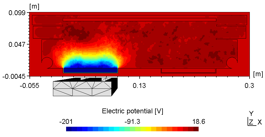
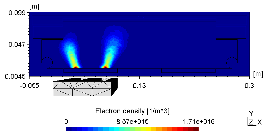
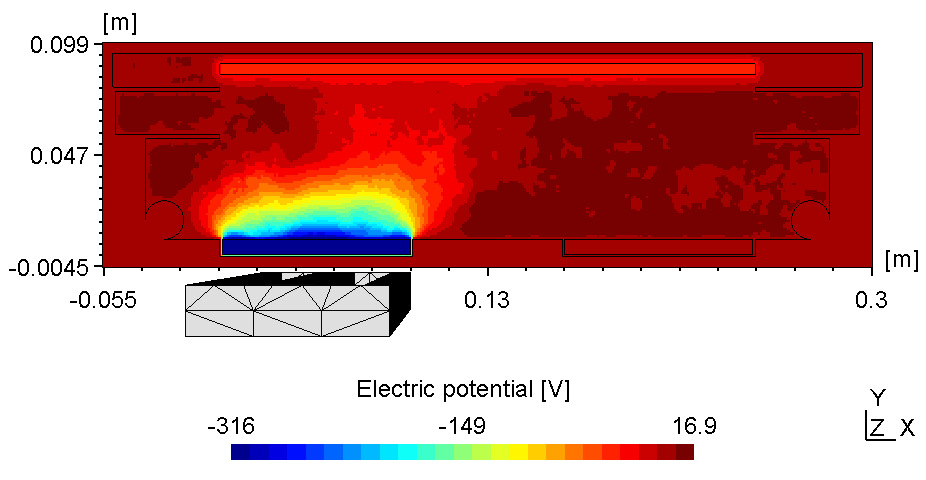
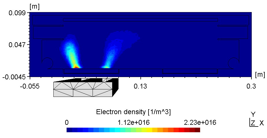
The plasma in a 2D set-up is not coupled and thus, more sensitive to the anode configuration. With the substrate on ground potentialthe right plasma is as bright as the left one (see figure 1).

Table 5.2: Electric potential (left) and electron density (right) during simulation with substrate on ground potential (0 V).

Electric potential	Electron Density

5.1.8 Substrate on floating potential

Here the left plasma is conductively connected to the ajacent chamber wall, the right one however is connected with the top of the chamber wall. Thus, with the substrate on floating potential some of the anodic surface is shielded causing the right plasma to fade (see figure 2). Due to the uncoupled electron drift current in a 2d setup this effect is even more pronounced. Thus, if using constant power the voltage can drop below ignition point causing the right plasma to diminish.

Table 5.3: Electric potential (left) and electron density (right) during simulation with substrate on floating potential.

Electric potential	Electron Density