DSMC and PICMC documentation

3.1.3.1 Functions to import data

There are three main functions for importing data:

• obj.read("input.pos", "name");
  Reads an input file in GMSH postprocessing format *.pos and stores it under the internal name name. If multiple files are loaded under the same name, they are automatically internally averaged. This feature is mostly being used for time-averaging over multiple data snapshots taken at different times.
• obj.merge("input.pos", "name");
  This command is used for combining multiple postprocessing files with different data coordinates into a single dataset. It is mostly being used for combining multiple files with e.g. individual particle positions taken at different timesteps into a trajectory plot.
• obj.append("input.pos", "name");
  The append command is used to append multiple postprocessing files into a time series.

3.1.3.2 Simple cut planes

A simple functionality, which is most frequently used, is to make a 2D cutplane from a 3D dataset, which is parallel to the coordinate axes. There are the following three options for that:

• obj.xy_plane(z0, delta_z, "method");
  Cutplane parallel to the X-Y axes at z coordinate z0 within a range for data points of \(z0\pm \delta_z\)
• obj.xz_plane(y0, delta_y, "method");
  Cutplane parallel to the X-Z axes at y coordinate y0 within a range for data points of \(y0\pm \delta_y\)
• obj.yz_plane(x0, delta_x, "method");
  Cutplane parallel to the Y-Z axes at x coordinate x0 within a range for data points of \(x0\pm \delta_x\)

The "method" parameter describes how to project data points onto the cut plane. There are three options:

• "nearest_neighbour"
  The nearest datapoint located in perpendicular direction within the search range is projected onto the cutplane.
• "average" All data points located in perpendicular direction within the search range are averaged, and the average value is taken at the position of the cutplane.
• "interpolate" The value is calculated by linear interpolation between two data points located on both sides of the cutplane within the search radius

3.1.3.3 General oblique planes and lineprofiles

Oblique cutplanes or can be created with the more general methods

obj.plane(x0, y0, z0,  x1, y1, z1,  x2, y2, z2,   delta, N, M, "method");
obj.line( x0, y0, z0,  x1, y1, z1,  delta, N,                  "method");

For a detailed description, please refer to this example.

3.1.3.4 Cylindrical cutplanes

2D cutplanes along a cylindrical surface can be obtained via

obj.cylinder(x0, y0, z0,  x1, y1, z1, r_cyl, delta, nl, nphi, "method");

Please refer to the example on cylindrical cutplanes for further explanation.

3.1.3.5 Output functions

The postprocessing module can create output files either in GMSH postprocessing format *.pos, Techplot format or VTK format. Depending on the type of data, the outputs can be either in scalar or vector format. For GMSH postprocessing files, there are the following options:

obj.write_pos_scalar("output.pos", "View title", expression);
obj.write_pos_vector("output.pos", "View title", 
                     expression_x, expression_y, expression_z);
obj.write_pos_scalar_binary("output.pos", "View title", expression);
obj.write_pos_vector_binary("output.pos", "View title", 
                     expression_x, expression_y, expression_z);
obj.write_pos_triangulate("output.pos", "View title", expression);

The first two commands produce GMSH *.pos files in ASCII format, which contain either scalar or vector data. The next two commands do the same but produce files in binary *.pos format, which is somewhat compressed in comparison to the ASCII format. The last command works only after a 2D cutplane operation and produces a triangulated view of scalar data, which means that they are represented as a triangulated surface.

Each command takes the name of the outputfile and the caption of the view ("View title") as arguments, followed by one or more arithmetic expressions. The expression parameters contain an arithmetic expression, which should be evaluated at the respective datapoints of the last operation (cutplane, lineprofile etc.). They could use the variables x, y, z, which represent the actual coordinates, and in case of cylindrical cutplanes also the variable phi, which represents the azimuth angle.

Additionally, it can contain any of the variable names specified under name in the import functions as well as their maximum and minimum value via name_max and name_min. If the imported quantity is a vector dataset, the individual components are accessible via name_x, name_y, name_z, and thereof, the maxima / minima are again accessible via name_x_max, name_x_min etc.

There is an additional category of output functions, where also the coordinates of the output data can be explicitely manipulated:

obj.write_pos_scalar_parametric("output.pos", "View title", 
                                x, y, z, expression);
obj.write_pos_scalar_binary_parametric("output.pos", "View title", 
                                       x, y, z, expression);
obj.write_pos_vector_parametric("output.pos", "View title", 
                    x, y, z, 
                    expression_x, expression_y, expression_z);
obj.write_pos_vector_binary_parametric("output.pos", "View title", 
                    x, y, z, 
                    expression_x, expression_y, expression_z);

These functions work in the same way as the functions described above, but take the coordinates x, y, z as additional input. The purpose is to transform the coordinates of the output data in order to e.g. give them a coordinate offset or to project them onto a cylindrical surface.

Output functions of scalar and vector data in Techplot and VTK format work in the sam way, their syntax representations are

obj.write_tec_scalar("output.dat", "View title", expression);
obj.write_tec_vector("output.dat", "View title", 
                     expression_x, expression_y, expression_z);
obj.write_vtk_scalar("output.vtp", "View title", expression);
obj.write_vtk_vector("output.vtp", "View title", 
                     expression_x, expression_y, expression_z);

For export of data in ASCII files (either *.txt or *.csv) the following functions are available:

obj.write_txt("output.txt", 
              ["col1", "col2", ...], [exp1, exp2, ...]);
obj.write_csv("output.csv", 
              ["col1", "col2", ...], [exp1, exp2, ...]);

Besides the name of the output file, these functions expect a list of column names and a list of expressions for the columns (obviously, both lists have to be of the same length). The expressions in the expression list can use the same variable names as described above.

Finally, there are output functions for time series (animations). In contrast to the previous output functions, they work not (yet) with arithmetic expressions but only with variable names, as were used in the "name" argument of the append command. If needed, additional input data sets can be computed via the commands create_scalar, create_vector as described in the data manipulation section.

obj.write_pos_time_steps_scalar("output.pos", 
                                "View title", "name");
obj.write_pos_time_steps_scalar_binary("output.pos", 
                                "View title", "name");
obj.write_pos_time_steps_vector("output.pos", 
                                "View title", "name");
obj.write_pos_time_steps_vector_binary("output.pos", 
                                "View title", "name");

3.1.4.1 Creation of new input data

Usually, the input data is obtained directly via the command obj.read("filename", "label");. In some cases it may be useful to create additional input data via an algebraic formula from the existing data. For this purpose, the following commands can be used:

• obj.create_scalar("new_label", expression);
  Create new scalar input data entry
• obj.create_vector("new_label", exp_x, exp_y, exp_z);
  Create new vector input data entry

In the example above, it is possible to plot the relative density distribution in % because of the existence of the view variable n_max. However it is not clear how to plot e.g. the relative flux distribution, since there is no obvious way to obtain the maximum value of n*v_z. By creation of a "flux" variable as new input entry, this problem can be solved (see example listing and data structure diagram below).

compiletime load "module_ppp.so";
PPP obj = {};

obj.read("density.pos",  "n");
obj.read("velocity.pos", "v");

obj.create_vector("flux", n*v_x, n*v_y, n*v_z);

obj.xy_plane(0, 10, "nearest_neighbour");

obj.write_pos_scalar_binary("flux-Z.pos", 
                            "Vertical flux [1/m^2 s]", flux_z);
obj.write_pos_scalar_binary("flux-Z-relative.pos", 
                            "Relative Vertical flux [%]", 
                            100*flux_z/flux_z_max);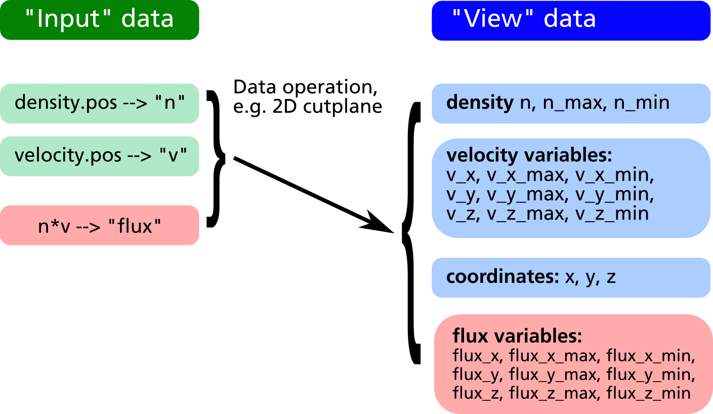

3.1.4.2 Reduction of input data

Let us assume we have 3D data of the density and velocity of evaporated atoms. In the XY-plane at Z=100 there is a substrate where the evaporated atoms can condensate.

First, in order to get the thickness profile on the substrate, the flux has to be extracted by multiplying density and z component of velocity in a cut-plane just below the substrate surface.

Second, let us assume the substrate is moving into Y direction, i.e. we have a dynamic deposition. In such cases, only the linescan of the profile in X direction averaged over Y is of relevance.

In order to do this, in prior versions of the post processing module it was required to make the 2D cut plane first, save it into a temporary POS file, load this POS file into a second post processing object and finally extract the line profile from there.

From version 2.4.3 on, there is the possibility of reducing the input data according to the last executed geometric operation, the command syntax is:

• obj.reduce();
  Reduction of input data space according to current arrangement of view data.

This allows for obtaining a line profile from 3D data in a much easier way:

compiletime load "module_ppp.so";
PPP obj = {};

aperture_width = 100;   # Aperture width on substrate in transport direction

obj.read("density.pos", "n");
obj.read("velocity.pos", "v");

# Define vertical flux component
obj.create_scalar("Fz", n*v_z);

# Make cut plane of data just below the substrate surface
obj.xy_plane(99.5, 10, "nearest_neighbour");  

# Reduce input data to cut-plane (this is the important command)
obj.reduce(); 

# Make another cut plane averaging over the aperture_width
# in order to get the line profile
obj.xz_plane(0, aperture_width/2, "average");

# Write line profile into TXT file
obj.write_txt("absorption_line.txt", 
              ["x", "avg_absorption", "rel_absorption"],
              [x, Fz, 100*Fz/Fz_max]);

3.1.4.3 Control of written data

Regarding the format of written data, there are the following possibilities:

• The coordinates, where the written data get plotted in POS files, can be explicitely specified
• It is possible to set a flag deciding whether to write data at a given coordinate point or not

The first option involves the following output methods:

• obj.write_pos_scalar_parametric("filename.pos", "Legend", x, y, z, expression);
• obj.write_pos_scalar_binary_parametric("filename.pos", "Legend", x, y, z, expression);
• obj.write_pos_vector_parametric("filename.pos", "Legend", x, y, z, exp_x, exp_y, exp_z);
• obj.write_pos_vector_binary_parametric("filename.pos", "Legend", x, y, z, exp_x, exp_y, exp_z);

The first two commands are for parametrized scalar plots (in ASCII and binary format, respectively), the second two commands are for vector plots. An example is given in the following listing.

compiletime load "module_ppp.so";

PPP obj = {};
obj.read("density.pos",  "n");
obj.read("velocity.pos", "v");
obj.xy_plane(100, 10, "nearest_neighbour");

# Plot density and flux side by side. A coordinate offset allows for
# loading both pos files into GMSH and have the cut planes non-overlapping

obj.write_pos_scalar_binary_parametric("density-2D.pos", "Density [1/m^3]", 
                                       x, y, z, n);
obj.write_pos_scalar_binary_parametric("flux-2D.pos", "Flux [1/m^3]", 
                                       x+200, y, z, n*v_z);

In order to control explicitely, which data point should be written and which should be omitted, there is the possibility to define a write_flag variable within the postprocessing object. This is demonstrated in the following:

compiletime load "module_ppp.so";

PPP obj = {
  write_flag: A>0;
};

obj.read("absorption.pos", "A");
obj.write_pos_scalar_binary("absorption-noZeros.pos", "Absorption [1/m^2 s]", A);

In a large 3D absorption file, non-zero values only occur at the intersection between volume grid and mesh elements of walls. Thus a large fraction of the POS file consists of zeros, which is a waste in memory consumption. With the above script, the write_flag variable forces the write routine to only output those values with non-zero absorption, i.e. A>0.

It is important to define write_flag with a colon and not to write write_flag = (A>0);. In the rvm scripting language, the colon means that the value of write_flag will be only computed on request according to the currently defined parameters on right side. With the regular "=" assignment operator, the value of the variable A will be required at the moment of the definition of write_flag, which is not the case in the above script.

It is also possible to combine multiple conditions e.g. in order to specify a certain coordinate range for output:

compiletime load "module_ppp.so";

PPP obj = {
  write_flag: (abs(x)<100) and (y>-50) and (y<150);
};

# ...

3.1.4.4 Convolution function

A convolution function has been implemented to operate on target absorptions plots in an attempt to model erosion profiles in MoveMag aplications. The primary approach here is to assume plasma and ion bombardment, respectively do not change with magnetron position which should be valid for small displacements vectors. Thus, we simply integrate over time the convolution of a time deviant, i.e. moving absorption plot with a stationary step function.

Table 3.1: Convolution over a target with moving source (racetrack)

Convolution and integration over time of moving source data with stationaly step function	Absorption plot (top) and convolution result (bottom) for a periodic oscillation in y

compiletime load "module_ppp.so";

PPP obj1 = {};

#Define velocity vector and integration time
float vx[4], vy[4], vz[4]; #[m/s]
float T = 4; #[s]

#Oscillation starting from center position
#Move 1s to left with 1 m/s, then 2 times to right accordantly, then left again.
vx[0] = -1;
vx[1] = +1;
vx[2] = +1;
vx[3] = -1;

obj1.read("absorption_Arplus_100.00us.pos", "val");

obj1.xz_plane(0.0088, 1, "nearest_neighbour");

obj1.reduce; #Operate on cut plane (2D) data set for better performance!

obj1.convolution(vx, vy, vz, T, 0);

obj1.write_pos_scalar_binary("absorption_Arplus_100.00us_convolution.pos", val);

3.1.4.5 Convolution with linear weighting

Entering '1' for the weighting flag enables a linear weighting scheme during convolution operation from 1 (no displacement) to 0 (maximum displacment). With this you can realize an interpolation between two or more states, i.e. magnetron positions, by merging the results from corresponding convolution operations together.

Table 3.2: Linear convolution examples with constant and linear weighting

Convolution with constant weighting	Convolution with linear weighting

3.1.4.6 Circular Convolution

For a 360° convolution over the plot center use the function 'convolution_circular()' as seen below. This function has been implemented to adress modeling of absorption profiles on rotating substrates.

compiletime load "module_ppp.so";

PPP obj1 = {};

obj1.read("absorption_Arplus_100.00us.pos", "val");

obj1.xz_plane(0.0088, 1, "nearest_neighbour");

obj1.reduce; #Operate on cut plane (2D) data set for better performance!

obj1.convolution_circular();

obj1.write_pos_scalar_binary("absorption_Arplus_100.00us_convolution.pos", val);

Table 3.3: Example of a circula convolution

Source data	After circular convolution

obj.create_scalar("variable_name", expression);
obj.create_vector("variable_name", expression_x, expression_y, expression_z);

result = obj.integrate(expression);
obj.identity();
obj.reduce();
obj.convolution(vx, vy, vz, T, interpolation);
obj.convolution_circular();