
DSMC and PICMC documentation
2022-02-17
2.1 Wall interaction model
The interaction between the gas phase and walls is designed with the aim to provide an interface for setting up arbitrary reaction chains with high flexibility. For meshed geometric boundaries, there is one common wall type, where reactions and particle sources can be attached. Additionally, it is possible to declare single-sided mesh surfaces as membranes. Membranes fulfill special purposes such as virtual particle sources in the simulation space, particle flow barriers or virtual surfaces for sampling of energy and angular flux distributions.
A wall is represented in the GMSH mesh file as one physical surface group. In the PIC-MC / DSMC simulation parameter file a wall is represented as a Border entry as shown in the following example:
block BORDER_TYPES: {
  # ...

  Border Inlet = {
    icodec =   2;                       # Codec number from meshfile
    type = "wall";                      # Alternative type: "membrane"
    T = PAR.T0;                         # Wall temperature
    reactions: {
      add_source("O2", 1, "Pa");
    };
    # Rel. dielectric permittivity (insulator only)
    # epsr = 1.0;

    # Voltage function (conductor, can be time-dependent)
    # vf = "VP*cos(2*PI*13.56e6*TIME)"; # Voltage function (conductor)

    # Counter electrode in case of relative potential
    # vf_coupling = "";
  };

  # ...
};
Each Border entry has the following common parameters:
icodec: Integer number specifying the physical surface group. This number is automatically extracted from the mesh file and should be only changed in special cases.1type: String constant which can be either"wall"or"membrane". A"wall"must be part of a 3D object of the mesh file, while the"membrane"is a virtual, single-sided (i. e. infinitesimal) surface which can be used to block orifices, insert additional particle sources or for sampling purposes.T: Floating point number specifying the wall temperature in K.reactions: { \... };: Within this block, wall reactions and particle sources can be specified. A detailed description is given in the following subsections.epsr: Optional floating point variable specifying the dielectric permittivity of a dielectric insulating object (e.g. a glass susbtrate) in case of a plasma simulation.vf: Optional string variable specifying a time-dependent voltage function.vf_coupling: Optional string variable specifying a counter electrode within systems of floating electrodes with built-in potential difference.
2.1.1 Particle sources
2.1.1.1 Constant sources
Particle sources can either have Maxwellian or Sputter type energy emission, or a given emission energy interval can be specified. The declaration syntax is add_source("species", amount, "unit");
Example:
add_source("O2", 50, "sccm");
add_source("Al", 10, "Pa");
Both commands declare a particle source. The first argument is the gas species to be created, the second argument the amount. The unit argument can be either "sccm" or "Pa" specifying a mass flow or pressure controlled source, respectively.
2.1.1.2 Sources with inscribed profile
For the source surface it may be required to have a non-uniform profile over the source surface.
An example is magnetron sputtering where the sputtering emission distribution from the cathode depends on the Ar+ ion bombardment profile. The Ar+ ion bombardment profile can be stored in an absorption plot by putting Arplus into the ABSORPTION plot list.
In a subsequent DSMC neutral transport simulation, e.g. in order to evaluate the film thickness profile of the sputtered material, there is now an easy way to use the Ar+ ion bombardment profile for defining the sputtering source:
add_source("Ti", 50, "sccm");          # Flow controlled Ti source
set_emission_sputter("Ti", 4.89, 1.0); # Sputtering with Ub = 4.89 eV
set_profile("Arplus-absorption.pos");  # Specify distribution profile
                                       # (e.g. ion flux profile from
                                       # previous plasma simulation)
The file Arplus-absorption.pos is a simulation output file. It can be either in cell resolution or in mesh resolution. Alternatively, a time-averaged file can be made from several absorption plots via post processing. In the set_profile command, the filename has to be given as relative path with respect to the location of the parameter file (in the example above, Arplus-absorption.pos must be in the same directory as the parameter file).
A more accurate way is to model the sputtering process within the PIC-MC plasma simulation by taking into account the angular and energy dependency of the sputtering yield. In this case, the desorption_XXX.pos files or their mesh plot equivalents can be taken as profile for the subsequent DSMC simulation. However the assumption that the local sputtering rate is proportional to the ion flux is a good starting approximation in most cases.
2.1.1.3 Vapor pressure source depending on surface temperature
In some cases, a source surface might have a temperature profile. This is especially relevant in connection with imported wall temperature distributions. In case of a pressure source - e.g. for an evaporation surface - the vapor pressure is temperature dependent. Most temperature-dependent vapor-pressure curves can be fitted with a simple exponential expression (with the temperature \(T\) given in Kelvin):
\[ p(T) = exp(-a/T + b) \](2.1)
The syntax of the temperature-dependent pressure source is:
add_vapor_source("species", a, b);The parameters a and b are the same as in Eq. (2.1) and are material dependent. For Aluminum, suitable values are a=36070 and b=24.469. Thus, a temperature-dependent Al evaporation source can be defined by:
add_vapor_source("Al", 36070, 24.469);2.1.2 Particle emission characteristics
Particles are emitted from walls for two possible reasons. Either a Particle source (section (sec:prep_particle_sources?)) is attached to the wall or a reaction involving reaction products takes place.
In both cases, the default behaviour is to emit particles with a Maxwellian velocity according to the given wall temperature and a \(\cos(\theta)\) like angular distribution. A Maxwellian distribution in 3D space is characterized by following distribution function in the velocity \(v\)
\[ f(v)dv = \sqrt{\frac{2 m^3}{\pi k^3T^3}} v^2 \exp\left(-\frac{mv^2}{2kT}\right)\](2.2)
where \(T\) is the temperature, \(k\) the Boltzmann constant, and \(m\) the molecular mass. When sitting at a wall surface, the velocity distribution function has to be multplied with the particle velocity \(v_z\) normal to the surface, since the arrival of fast particles is then statistically emphasized. In the software implementation, the particle velocities of diffusely reflected or generated particles with Maxwellian distribution are generated as follows in cylindric coordinates \((r,\phi, z)\) with the \(z\) coordinate aligned parallel to the surface normal:
\[\begin{aligned} v_z &= \sqrt{-\frac{2kT}{m}\ln(R\#)}\nonumber\\ v_r &= \sqrt{-\frac{2kT}{m}\ln(R\#)}\nonumber\\ \phi&= 2\pi R\# \\ \vec{v}_\textrm{Emitted} & = v_z \hat{n} + v_r\cos(\phi)\hat{t_1} + v_r\sin(\phi)\hat{t_2},\nonumber \end{aligned}\](2.3)
with \(R\#\) being a random number between \([0, 1[\) and \(\hat{n}, \hat{t_1}, \hat{t_2}\) being the surface normal and normalized tangential vectors. If this algorithm is performed for reflected particles in a closed gas volume, the gas will be everywhere in thermal equilibrium with the wall and will have a Maxwellian distribution according to the wall temperature.
It is possible to modify the behaviour of generated particles by supplying an additional command just after the last wall command involving reaction products (either after the last source or reaction).
2.1.2.1 Maxwellian distribution with alternative temperature
If required it is possible to emit particles with Maxwellian distribution with a different temperature than specified in the wall properties. For this purpose, there is a function set_emission_maxwell which takes the desired temperature as argument:
set_emission_maxwell("species", temperature);2.1.2.2 Source of sputtered particles
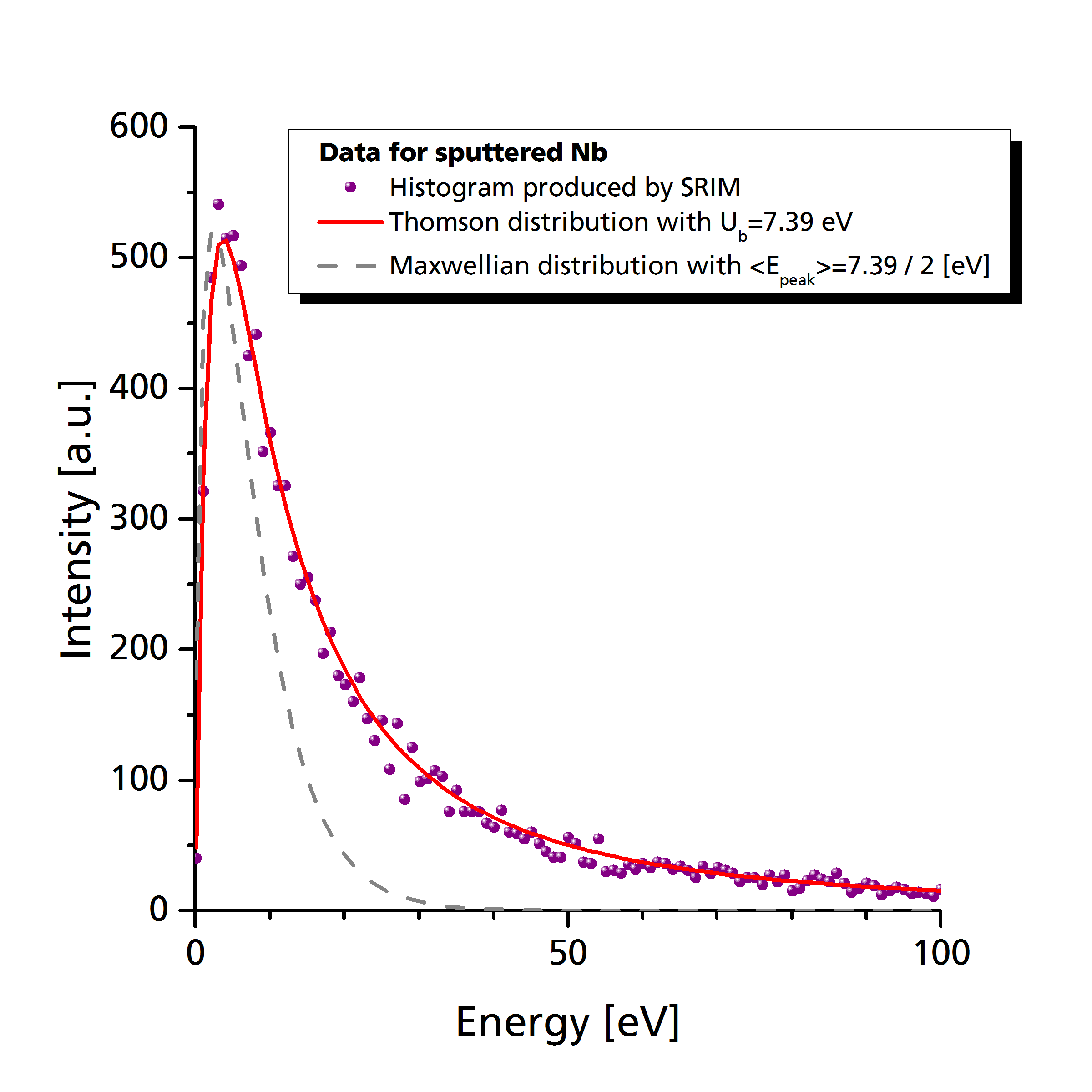
A sputter process results from random ballistic collisions between atoms inside the target material. The distribution of sputtered species is non-thermal. A thorough discussion on that topic is given in the book Sputtering by Particle Bombardment by (Behrisch and Eckstein 2007). The distribution function of sputtered particles has been discussed in (Thompson 1981) yielding following relation:
\[ f(E,\theta) \propto \frac{\cos(\theta)}{E^{2-2m}\left(1+U_b/E\right)^{3-2m}}\](2.4)
Here, \(m\) is a parameter describing the interatomic potential between target atoms. Assumption of the hard-sphere approximation leads to \(m \rightarrow 0\). The software implementation uses this simplification within the function set_emission_thompson together with an angular distribution function \(f_\alpha(\theta)\), which depends on a parameter \(\alpha\):
\[f(E,\theta) \propto \frac{E}{\left(E+U_b\right)^3}\times f_\alpha(\theta)\](2.5) \[f_{\alpha}(\theta) = \left\{ \begin{array}{ll} \cos^{\alpha}(\theta); & \alpha \ge 0\\ \cos(\theta) \left(1+\alpha\cos^2(\theta)\right); & \alpha < 0 \end{array} \right.\](2.6)
The angular distribution for negative values of \(\alpha\) is an empirical formula for off-axis sputtering characteristics taken from (Yamamura, Takiguchi, and Ishida 1991). It could be relevant for polycrystalline target materials and in case of low ion energies (Wehner and Rosenberg 1960). For performing ballistic simulation of the sputter process in targets, there is a free software called SRIM, which can produce sputter yields, velocity and angle distribution of sputtered particles as well as implantation profiles for arbitrary target compositions and ion impact. The software implementation includes both formula for the angular distribution function, which are selected according to the parameter \(\alpha\).
As can be seen in the following graph (Pflug et al. 2014), the distribution of sputtered particles decays much slower with energy than e.g. a Maxwellian distribution with the same peak energy (The peak energy in case of a sputter distribution is located at \(E_\textrm{peak} = U_b/2\)).
One conceptual problem of the above distribution function by Thompson is that there is no upper limitation regarding the kinetic energy of sputtered species. Generation of particles with arbitrarily high kinetic energy is problematic since they potentially violate numerical constraints with respect to time step and cell spacing.
A practical solution is based on the maximum fraction \(\lambda\) of energy which can be transferred from an impinging ion with mass \(m_i\) to a target atom with mass \(m_t\) by perpendicular collision[^footnote_thompson_2],
\[\lambda = \frac{4 m_i m_t}{\left(m_i+m_t\right)^2}\](2.7)
With \(E_i\) as the energy of impinging ions it is reasonable to assume that the energy of sputtered atoms can be no higher than \(\lambda\times E_i\). Thus, in the DSMC / PICMC software implementation, \(\lambda\times E_i\) is used as upper limit of the kinetic energy of sputtered particles. The accordant function for the Thompson distribution is
set_emission_thompson("species", Ub, alpha, E_ion, m_ion);The parameters are as follows:
"species"--> the name of the sputtered speciesUb--> The binding energyalpha--> The parameter $\alpha$ determining the angular distributionE_ion--> The kinetic energy of impinging ionsm_ion--> The relative molecular mass of impinging ions
The latter two parameters are used to compute the above mentioned recoil factor \(\lambda\) from Eq. (2.7). The simplified Thomson distribution can be analytically integrated, thus in the practical implementation the energy is taken via
\[E = \frac{U_b}{1-\sqrt{R\#}} - U_b\](2.8)
Again, \(R\#\) is a random number within \([0,1[\). The emission angle is created via
\[\theta = \left\{\begin{array}{ll} \arccos\left(\left(1-R\#\right)^{\frac{1}{\alpha+1}}\right); & \alpha \ge 0\\ \arccos\left(\sqrt{\frac{\sqrt{1+\alpha(2+\alpha)(1-R\#)}-1}{\alpha}}\right); & \alpha < 0 \end{array}\right.\](2.9)
If the random number yields \(E > \lambda E_i\) then the value is dropped and the calculation is repeated for another random number \(R\#\).
Note: In former versions (before 2.4.2.8) the Thompson distribution function was generated via
set_emission_sputter("species", Ub, alpha);Here, the cut-off energy was internally hard-wired as \(E_\textrm{cutoff} = 100\times U_b\). This function still works, but we recommend using the newer function set_emission_thompson instead, where the cut-off energy can be freely specified. Especially in case of sputtered species deposited onto a substrate it turned out that unrealistically high values of the cut-off energy can lead to significant deviations in their mean energy.
2.1.2.3 Uniform energy distribution within a given interval
For a uniform distribution within an energy interval between E0…E1, the following function can be used:
set_emission_energy("species", E0, E1, alpha);The angular distribution as a function of the parameter $\alpha$ is the same as in case of sputtered particles (see previous section).
Example: Niobium sputter source
# Constant sputter rate equivalent to 50 sccm particle flux
add_source("Nb", 50, "sccm");

# Sputter emission with Ub = 7.39 eV and cosine index 1.5
set_emission_sputter("Nb", 7.39, 1.5);
2.1.2.4 Particle emission distribution by user defined histogram
If the built-in particle emission profiles are not sufficient, there is also the possibility of implementing a user-defined distribution function via histogram data files. The histogram data files must have the same format as the files resulting from sampling energy and angular distribution, i.e. four columns comprising
- Energy [eV]
- Theta [°]
- Phi [°]
- Scalar intensity
There are the following four options:
- Energy only distribution function
set_emission_histogram_E("species", alpha, hist_filename);
Here, only the first and fourth column of the histogram file (energy and intensity) will be taken into account. For the angular distribution function, the parameteralphahas the same meaning as shown above (see section (sec:prep_sputter_source?)). - Angular only distribution function
set_emission_histogram_A("species", temperature, hist_filename, ex, ey, ez);
Here, the first column of the histogram file is ignored; relevant are columns 2-4 (theta and phi angle as well as intensity). The angles are to be given in degree. Additionally, a unit vectorex, ey, ezis to be specified, this vector defines the direction, where the azimuth angle is zero. - Separated energy and angular distribution functions
set_emission_histogram_EA("species", hist_E_filename, hist_A_filename, ex, ey, ez);
Here, energy and angular distribution function are both to be specified and treated independently. - Correlated energy and angular distribution function
set_emission_histogram_Corr("species", hist_filename, ex, ey, ez);
This function uses only one histogram file, where energy and angular columns are both included, i.e. energy and angular distributions are correlated.
2.1.2.5 Particle emission distribution by user defined functions
Instead of providing emission distribution functions as histogram files, they can be also applied as analytic formula. There are the following options:
- Energy distribution function
set_emission_function_E("species", alpha, eMax, ne, formula);
The energy distribution function for the emitted"species"is defined on an energy interval0...eMaxwithnebeing the number of slots. The energy unit used to specify the range is eV. The parameteralphaspecifies the angular emission profile as specified in section (sec:prep_sputter_source?). The analytic function is specified via parameterformula, which can contain an analytical formula withEbeing the energy in eV. - Angular distribution function
set_emission_function_A("species", T0, nTheta, nPhi, formula, ex, ey, ez);
This specifies an angular distribution function while assuming an Maxwellian energy distribution function according to the temperatureT0. The resolution of the angular distribution function is defined by the number of slots,nThetafor the polar angle andnPhifor the azimuth angle. The analytical function in parameterformulamay contain the variablesTHETA(range: 0-90° in degree),theta(range: \(0\ldots\pi\)),PHI(range: 0-360° in degree) orphi(range: \(0\ldots 2\pi\)). The parametersex, ey, ezrepresent a vector which defines the direction where \(\phi=0\). - Independent energy and angular distribution functions
set_emission_function_EA("species", eMax, ne, formula_E, nTheta, nPhi,
formula_theta_phi, ex, ey, ez);
This function - as a combination of the two previous functins - allows to set independent energy and angular distributions. The energy distribution function for the emitted"species"is defined on an energy interval0...eMaxwithnebeing the number of slots. The energy unit used to specify the range is eV, and the analytical formula as a function ofEis specified via parameterformula_E. The resolution of the angular distribution function is defined by the number of slots,nThetafor the polar angle andnPhifor the azimuth angle. The analytical function parameterformula_theta_phimay contain the variablesTHETA(range: 0-90° in degree),theta(range: \(0\ldots\pi\)),PHI(range: 0-360° in degree) orphi(range: \(0\ldots 2\pi\)). The parametersex, ey, ezrepresent a vector which defines the direction where \(\phi=0\). - Correlated energy and angular distribution function
set_emission_function_Corr("species", eMax, ne, nTheta, nPhi,
formula, ex, ey, ez);
This function allows to specify a correlated energy and angular distribution function. The energy distribution function for the emitted"species"is defined on an energy interval0...eMaxwithnebeing the number of slots and the energy unit in eV. The resolution of the angular distribution function is defined by the number of slots,nThetafor the polar angle andnPhifor the azimuth angle. The distribution function specified informulacan contain all variablesE, THETA, PHI, theta, phias specified above.
2.1.2.6 Specifying energy loss functions
In case of e.g. reflected neutrals from ion impact or reflected high energetic electrons, where a certain energy loss occurred in the material, the energy distribution of the reflected species is not given as a function of absolute energy. Instead, there is a distribution function for either the absolute or the relative energy loss. Such cases can be specially treated:
- Relative energy loss function
set_energy_loss_rel("species", formula);
A relative loss function occurs e.g. for fast reflected neutrals resulting from ion impact on a target. Here, the ratio between impact and emitted energy depends e.g. on a mass ration between ion and target atom and thus, the loss energy distribution is defined on a relative scaleE=0...1. This function uses a resolution of 1000 slots of the relative energy scale by default. The parameterformulamay depend on the variable E, which - in this case - is not the absolute energy but a relative one (E=0…1), where E=1 corresponds to the impact energy. - Absolute energy loss function
set_energy_loss_abs("species", eMax, ne, formula);
This realizes an absolute loss function. One scenario may be a high energetic electron impinging on a surface thereby inducing some Auger excitation or other energy loss mechanism in the material which would substract an absolute loss energy from the electron. In this case, the energy range is E=0...eMax with the unit in eV, and the number of slots is specified in thenEparameter.
In these energy loss functions, the direction of the reflected particle is currently set specularly with respect to the impinging particle (even if e.g. the species changed from ion to neutral). In future versions this might be modified e.g. by specifying an angular cone for the reflected particle.
Example: In plasma simulations, the creation of fast reflected neutrals by ion impact can be realized as follows:
add_plain_reaction("Arplus", 1, 1, ["Ar", "e"], [1, 0.1]);
set_emission_function_E("e", 1.0, 10, 100, exp(-((E-5)^2)/2));
set_energy_loss_rel("Ar", E>0.35);
In this example, an Arplus ion impinging onto a surface results in an electron with a secondary electron yield of 0.1 (10%) and a neutral Ar atom2 with a yield of 100%. From the reflected neutral (Ar) the relative loss energy distribution is set to E>0.35. In the relative scale E=0...1 this evaluates to 1 of E>0.35 and 0 if E<=0.35. It means that the energy of the reflected Ar is reduced by 35% or more in comparison with the impact energy of the ion. In other words: The energy loss is equally distrbuted between 35% and 100% (The energy distribution of the secondary electron is set as Gaussian function centered around 5 eV, but this is not important, here).
2.1.3 Wall temperature distribution
A non-trivial temperature distribution on a wall is especially used in combination with a vapor pressure dependent particle source in order to get a more realistic behavior of e.g. large evaporation sources.
In order to define a temperature distribution rather than a single fixed temperature, the following command has to be used:
add_temperature("temperature_distribution.txt");The temperature distribution file format is currently according to Comsol-generated temperature output files. The format is as follows:
- First line: Title (will be ignored)
- Next lines: Seven columns of numbers separated by TAB or whitespace with following meaning:
<Facet> <Point> <X> <Y> <Z> <Element> <Temperature [K]>Only the (X, Y, Z) coordinates and the temperature will be read in, the other columns will be ignored.
The temperature can be defined at arbitrary points within the simulation volume, there is no specific ordering of the points required. Upon initialization, for each mesh element the nearest point of the temperature distribution is chosen and the respective temperature is put into the mesh element.
2.1.4 Plain reactions
A plain reaction can be particle absorption or particle transformation with a given contant sticking coefficient or reaction probability. There is no wall state or surface coverage involved. Reactions which consider the actual surface coverage with different surface materials are described under surface chemistry reactions below. Possible plain reactions are listed in the following:
2.1.4.1 Simple absorption with sticking coefficient
The simplest type of surface reaction is the absorption of an arriving species based on a constant absorption probability or sticking coefficient of a given species:
add_absorption("species", sticking_coefficient);Example:
# Define a pumping surface for Ar and H2
add_absorption("Ar", 0.2);
add_absorption("H2", 0.05);
2.1.4.2 Specular reflection
While the default behaviour of a species impinging onto a surface is diffuse reflection, it is also possible to specify a specular reflection with a given probability via
add_specular_reflection("species", probability);In most cases, specular reflection is not going to happen in real; however, this functionality is useful for defining symmetry planes.
2.1.4.3 Plain reaction with sticking coefficient and reaction products
This more generalized syntax allows to specify particle absorption in combination with reaction products. The syntax and parameters are as follows.
add_plain_reaction("species", flag, probability,
["rp1", "rp2", ...], [n1, n2, ...]);- “species”: Incoming gas species such as
"Ar"or"H2" - flag: Can be 0 or 1. A value of flag==1 means that the incoming species is absorbed, if flag==0 it is reflected at the surface.
- probability: A value between [0..1] specifying the reaction probability.
- [“rp1,” “rp2,” ..]: A comma-separated list of reaction products (use
[], if no reaction products are involved) - [n1, n2, …]: The respective yields of the reaction products
Example 1: SiH4 -> Si (film growth) + 2 H2 (reaction products given back to the gas volume) with a sticking coefficient of 50%
add_plain_reaction("SiH4", 1, 0.5, ["H2"], [2]);Example 2: Secondary electron generation with secondary electron coefficient \(\gamma=0.1\) by ion impact \(Ar^+ \rightarrow Ar + \gamma e^-\)
add_plain_reaction("Arplus", 1, 1, ["Ar", "e"], [1, 0.1]);The emission characteristics of reaction products is by default Maxwellian with a \(\cos(\theta)\) like angular distribution. In order to change this behaviour, the same commands for specifying the emission characteristics as in the particle sources can be used.
Example 3: Sputtering with Ar+
add_plain_reaction("Arplus", 1, 1, ["Ar", "e", "Nb", "Ominus"],
                                   [1, 0.1, 5, 0.04]);

# Electrons are perpendicularly emitted with energies between 0..10 eV:
set_emission_energy("e", 0, 10, 100);

# Nb is sputtered with Ub=7.39 eV and alpha=1.5
# As incident ions, Ar+ with an energy of 300 eV are assumed
set_emission_thompson("Nb", 7.39, 1.5, 300, 40);

# Set sputter energy distribution also for Ominus
set_emission_thompson("Ominus", 4.5, 1.5, 400, 40);
2.1.5 Secondary Electron Emission Yield
According to Zalm and Beckers (1985), there ary two mechanisms for electron ejection upon ion bombardment:
- Potential Emission: If the ion neutralization energy exceeds twice the electron work function of the material, electron emission is possible. The secondary electron emission yield resulting from this mechanism is energy dependent and applies for rather low ion incident energies up to a few 100 eV.
- Kinetic Emission: At higher energies, electron emission by direct ionization of metal atoms by the ion projectile and/or by energetic recoils becomes important. This mechanism becomes relevant for ion incident energies beyond 1 keV.
Given the relevant energy range, only the first mechanism seems relevant for magnetron sputtering. The secondary electron emission coefficient for potential emission can be calculated via Eqn. (2.10).
\[\gamma_\textrm{PEE}\approx 0.2\times \frac{0.8 E_i - 2\phi}{\epsilon_i}\](2.10)
- \(E_i\) = Ionization energy of the ion (= 15.8 eV for Ar+)
- \(\phi\) = Electron work function of the metal
- \(\epsilon_i\) = Fermi energy of the electrons within the metal
In the following, representative numerical values are given. Most of the values are taken from the following sources:
- Table of fermi energies from http://hyperphysics.phy-astr.gsu.edu/hbase/tables/fermi.html#c1 from the Hyperphysics project (University of Georgia)
- Wikipedia article about work function
| Metal | Work function [eV] | Fermi energy [eV] | ISEE for Ar+ (15.8 eV) | ISEE for O2+ (12.06 eV) |
|---|---|---|---|---|
| Ag | 4.63 | 5.49 | 0.123 | 0.014 |
| Al | 4.163 | 11.7 | 0.073 | 0.023 |
| Cu | 4.53-5.10 | 7.00 | 0.070-0.1022 | 0.0 - 0.017 |
| Ti | 4.33 | 4.556 | 0.175 | 0.043 |
2.1.6 Energy and angular dependency of reactions and particle yields
2.1.6.1 Energy dependent reaction probability
If reactions have an energy-dependent reaction probability, this can be defined via the function
set_probability_function(E0, E1, nE, function);This function is to be put just after the last reaction definition, and the parameters are as follows:
- E0, E1: Defines the energy interval [E0, E1]; the unit is eV.
- nE: The number of sub-intervals within [E0, E1];
- function: Functional expression, where the energy can be used as variable E
If the actual particle energy E is outside of the [E0, E1] interval, the probability values at E0, E1 will be taken for E<E0, E>E1, respectively.
Example: In McRae and Caldwell (1976), a detailed measurement of the electron reflection behaviour at Copper surfaces is shown in the following graph.
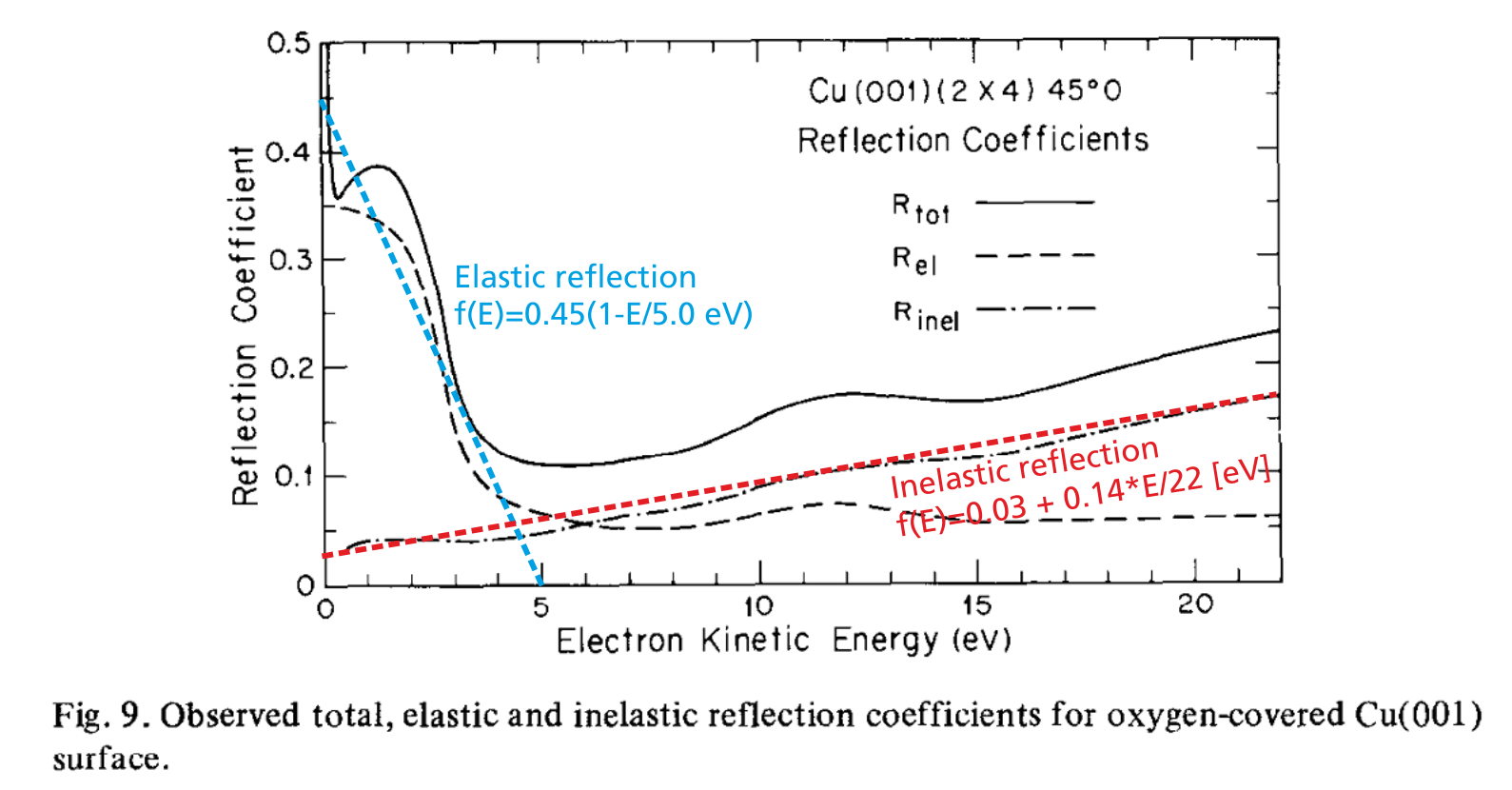
As can be seen, there is an elastic and an inelastic reflection probability curve; both curves can be approximated in first order by a linear function. In order to use these behaviour in PIC-MC simulations, the following plasma-wall interaction definition would be appropriate:
  add_plain_reaction("Arplus", 1, 1, ["Ar", "e"], [1, 0.1]);
  set_emission_energy("e", 0, 10, 100);

  add_specular_reflection("e", 1.0);
  set_probability_function(0, 5, 20, 0.45*(1-E/5));
  add_absorption("e", 1.0);
  set_probability_function(0, 22, 100, 1-(0.03+0.14*E/22));
The upper part of the code defines the emission of secondary electrons upon impact of positive ions. The reflection behaviour of low-energy electrons is defined in the lower four lines. First, a specular reflection is added with 100% probability. Afterwards, the energy-dependent probability function is applied. The resulting reaction probability will be the probability given in the add_specular_reflection function multiplied with the probability function (see also blue line in Fig. 6) given in the next command.
Since inelastic reflection is the default behaviour of all surfaces unless other reactions are specified, there is no set_inelastic_reflection command implemented. Instead the inverse process, i. e. the electron absorption at the wall is specified. Consequently, the probability function of the absorption is the inverse probability of the inelastic reflection probability (shown as red line in Fig. 6).
2.1.6.2 Energy dependent yield
If we have an energy-dependent yield of reaction products, it is better to use a yield function instead of the reaction probability. Its syntax is
set_yield_function("species", E0, E1, nE, function);The parameters are as follows:
species: Name of reaction product, whereof the yield energy dependency should be specifiedE0, E1: Energy interval of interestnE: Number of points within energy intervalfunction: Arithmetic expression, where the variableEcan be used for energy
The yield function will be multiplied to the yield given in the reaction product vector. All energy values are to be specified in (eV).
An example is the sputtering yield of Ti by Ar+ impact, whereof an empirical yield formula can be constructed from the data in (Ranjan et al. 2001) as follows:
\[Y(E) = 0.01085 (E/(1 eV)-118)^{2/3} (E \ge 118\textrm{ (eV)})\](2.11)
This case can be represented in the following way:
add_plain_reaction("Arplus", 1, 1, ["Ar", "e", "Ti"],
                                   [1,    0.1, 1]);
set_emission_thompson("Ti", 4.89, 1.0, 400, 40);
set_yield_function("Ti", 0, 1000, 1000,
                   (E>118) ? 0.01085*(E-118)^(2/3) ! 0);
It has to be noted that the yield function only affects the yield for the species Ti, while the yields of Ar and e are unaffected. In contrast, set_probability_function would affect the probability of the entire reaction by a multiplicative probability function; in the current scenario, this would be of no use.
2.1.6.3 Energy and angular dependent yield
In some cases, e.g. in sputtering processes, the number of emitted particles also depends on the angle of the impinging ion. In such cases, the yield of reaction products depends on both, the impinging particle energy and its angle. In such cases, the following function can be used to describe the energy and angular yield dependency:
set_yield_function_2D("species", E0, E1, nE, nTheta, function);The parameters are as follows:
species: Name of reaction product, whereof the yield energy dependency should be specifiedE0, E1: Energy interval of interestnE: Number of points within energy intervalnTheta: Number of points for interval of polar angle \(\theta\)function: Arithmetic expression, where the variablesE,THETAcan be used for the energy and polar angle, respectively. The energy unit is (eV), the angular unit is radian in the range \([0,\ldots,\pi/2[\).
A simplified interface for typical cases is
set_yield("species", function);Here, the energy range is predetermined to \([0,\ldots,1000]\) eV and the angular range is divided into 20 intervals. These settings should be appropriate e.g. for most sputtering processes.
Examples for energy-dependent sputter yields can be found in literature, e.g. in (Behrisch and Eckstein 2007) the fitting formula of Eq. (2.12) is proposed.
\[Y(E) = q \frac{0.5 \ln(1+1.2288 \epsilon)}{\epsilon+0.1728\sqrt{\epsilon}+0.008\epsilon^{0.1504}}\times \frac{\left(E_0/E_{th}-1\right)^\mu}{\lambda+\left(E_0/E_th-1\right)^\mu}\](2.12)
Fur further explanation please refer to chapter 3.2 in Behrisch and Eckstein (2007). An example curve can be generated via the following script:
float qq      = 4.8957;
float f_eps   = 8.56428*10^4;
float E_th    = 25.019;
float mu      = 1.8291;
float lambda  = 0.3152;

float E       = 200;

float sigma -> (E <= E_th) ? 0 !
               qq/2 * ln(1+1.2288*E/f_eps) /
               (E/f_eps+0.1728*sqrt(E/f_eps)+0.008*(E/f_eps)^(0.1504))*
               (E/E_th-1)^mu/(lambda+(E/E_th-1)^mu);

for(E=0; E<=1000; E=E+10) out "$(E)  $(sigma)\n";
The parameters at the beginning are chosen in accordance to the species involved, in the above example it is sputtering of Ti by Ar+. The script can then be executed with:
rvm sputter_yield.rIn order to integrate such curve into a simulation case, it is recommended to include a separate block into the parameter file immediately before block BORDER_TYPES { ...:
block wall_reaction: {
  float qq=4.8957, f_eps  = 8.56428e4, E_th = 25.019,
        mu=1.8291, lambda = 0.3152;

  show_reaction_message("Plasma-wall model with Ar+ sputtering on Ti, SEY=8%");
  add_plain_reaction("Arplus", 1, 1, ["Ar", "e", "Ti"], [1, 0.08, 1]);
  set_emission_energy("e", 0, 10, 100);
  set_emission_thompson("Ti", 4.89, 1.0, 300, 40);
  set_yield_function("Ti", 0, 1000, 1000,
                     (E <= E_th) ? 0 !
                     qq/2 * ln(1+1.2288*E/f_eps) /
                     (E/f_eps+0.1728*sqrt(E/f_eps)+0.008*(E/f_eps)^(0.1504))*
                     (E/E_th-1)^mu/(lambda+(E/E_th-1)^mu)
                     );

  add_absorption("e", 1);
}; # end of block wall_reaction
This block includes sputtering of Ar+ on Ti with a secondary electron yield of 8%. The sputtering yield for Ti is first set to 100% but later multiplied with the yield function below. In the respective physical surface definitions, this set of plasma-wall reaction can be applied as follows:
  Border Target = {
    icodec = 1;
    type   = "wall";
    T      = PAR.T0;
    vf     = "-VP";
    reactions: { PAR.wall_reaction; };
  };
2.1.7 Surface chemistry reactions
With plain reactions (section (sec:prep_plain_reactions?)), particle absorptions and transformations are defined without considering the state of the surface. A more advanced approach allows to define similar reactions in dependency of the actual surface material coverage. Fig. 2.3 shows an example of a surface coated with two different material components, which is exposed to the gas and/or plasma.
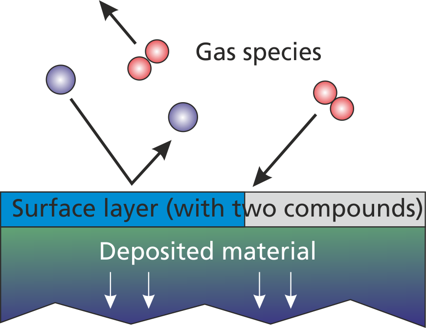
According to this representation, the advanced surface chemistry model considers three different regions:
- The gas phase and/or plasma
- The first atomic layer of the surface
- The deeper atomic layers which are in total representing the deposited layer material.
As already indicated, the surface layer and the deposited layer consists of multiple material compounds. A reasonable reactive model should comprise at least two different surface materials e. g. "Al" as metallic aluminum and "AlOx" as metal-oxide in a reactive deposition model.
2.1.7.1 Specification of wall materials and initial coverages
If we stick to the reactive AlOx deposition model, the first step is to declare two different names for the metal and metal-oxide:
add_material("Al", 1e19);
add_material("AlOx", 1e19);
set_initial_coverage("AlOx", 0.5);
The involved commands are
- Declare material name with bond density
add_material("material_name", bond_density); - Declare initial surface coverage of a material
set_initial_coverage("material_name", initial_coverage);
The bond_density parameter represents the surface density of bond sites of the material in (1/m2). For realistic molecular distances, the bond density typically is in the 1019 (1/m2) range. However it is possible to chose a smaller value in the simulation (e. g. 1017) in order to speed things up. If the wall is in equilibrium with the gas/plasma, the actual bond density has no influence on the result - it only influences the time required to reach the equilibrium state.
Note: Different bond density values for different materials are currently not yet supported and lead to undefined behaviour.
In order to get the deposition in the right unit you need to calculate the bond density depending on your material. The example calculation for AlOx is the following:
\[\begin{aligned} \rho_{Al_2O_3} & = 3.94 \textrm{ g cm}^{-3}\\ m_{Al_2O_3} & = 102\textrm{ u} = 1.7\times 10^{-22}\textrm{ g}\\ \rho_{Al_2O_3}^{'} & = \rho / m = 2.3\times 10^{22}\textrm{ cm}^{-3} = 2.3\times 10^{28}\textrm{ m}^{-3}\\ \rho_{Al_2O_3}^{''} & = {\rho^{'}}^{2/3} = 8\times 10^{18}\textrm{ m}^{-2}\\ \rho_{AlOx}^{''} & = 2\times\rho_{Al_2O_3}^{''} = 1.6\times 10^{19}\textrm{ m}^{-2} \end{aligned}\]
In the example given above it is sufficient to specify the initial coverage of only one material, e. g. AlOx. The coverage of Al will be automatically adjusted in a way that the sum of all coverages is 1.0. This works also for more than two materials.
Example:
add_material("Ti", 1e19);
add_material("TiO", 1e19);
add_material("TiO2", 1e19);
set_initial_coverage("TiO2", 0.9);
Here, the surface consists by 90% of "TiO2" (i. e. it is almost fully oxidized). The remaining 10% of the surface coverage is equally distributed amongst "TiO" and "Ti". If we write
add_material("Ti", 1e19);
add_material("TiO", 1e19);
add_material("TiO2", 1e19);
set_initial_coverage("TiO2", 0.9);
set_initial_coverage("TiO", 0.1);
then the initial coverage of "Ti" will be zero.
2.1.7.2 Surface reaction involving no deposition
The syntax for a surface reaction withou deposition - such as a surface oxidation - is shown in the following.
add_surface_reaction("species", flag, amount, probability,
                     "material_before", "material_after",
                     ["rp1", "rp2", ...], [n1, n2, ...]);
The parameters are
- species: String specifying the gas species
- flag: Specifies, if gas particle is absorbed (flag==1) or not (flag==0)
- amount: Number of gas particles required to accomplish one reaction (can be non-integer)
- probability: The reaction probability
- material_before, material_after: Strings specifying the required initial surface material and resulting surface material.
- [“rp1,” “rp2,” …], [n1, n2, …]: Reaction products and their amounts. As always their emission characteristics is Maxwellian by default and can be modified via
set_emission_sputter, set_emission_energyetc.
Still sticking to the reactive AlOx example, the oxidation of Aluminum can be described by Al + 0.75 O2->AlOx. The number 0.75 comes from the chemical formula Al2O3 of aluminum oxide.4 Translated to the command syntax and assuming a reaction probability of 50%, this yields
add_surface_reaction("O2", 1, 0.75, 0.5, "Al", "AlOx", [], []);2.1.7.3 Surface reaction involving deposition
While the surface oxidation of Al described above leads to a change in the surface material coverage, it does not increase the deposited film thickness. In contrast, if metallic Al is absorbed on the surface this leads to film growth. For that purpose, a modified syntax is required:
add_surface_deposition("species", amount, probability,
                       "material_before", "material_after", "material_deposited",
                       amount_deposited, ["rp1", ...], [n1, ...]);
Here, an additional parameter material_deposited describes the material component which contributes to the deposition zone. With the parameter amount_deposited the amount of surface sites per reaction can be controlled. There is no flag for the incoming gas species, since it is assumed that for a deposition process it will be always absorbed. Thus, the complete reactive AlOx example would look like follows (for Al with a deposition probability of 100%):
add_surface_reaction("O2", 1, 0.75, 0.5, "Al", "AlOx", [], []);
add_surface_deposition("Al", 1, 1.0, "Al", "Al", "Al", 1, [], []);
add_surface_deposition("Al", 1, 1.0, "AlOx", "Al", "AlOx", 1, [], []);
Please note that surface oxidation by "O2" only works if there is a non-zero metal fraction of "Al" present at the surface. "Al" deposition works for both possible surface materials.
2.1.7.4 Surface cover deposition
Many deposition reactions such as deposition of sputtered metal work equally on all possible surface materials. In all of these cases, the deposited metal “covers” the actual surface layer component and replaces it by itself. The surface layer component will then contribute to the deposited film. A visualization of this process is given in Fig 2.4.
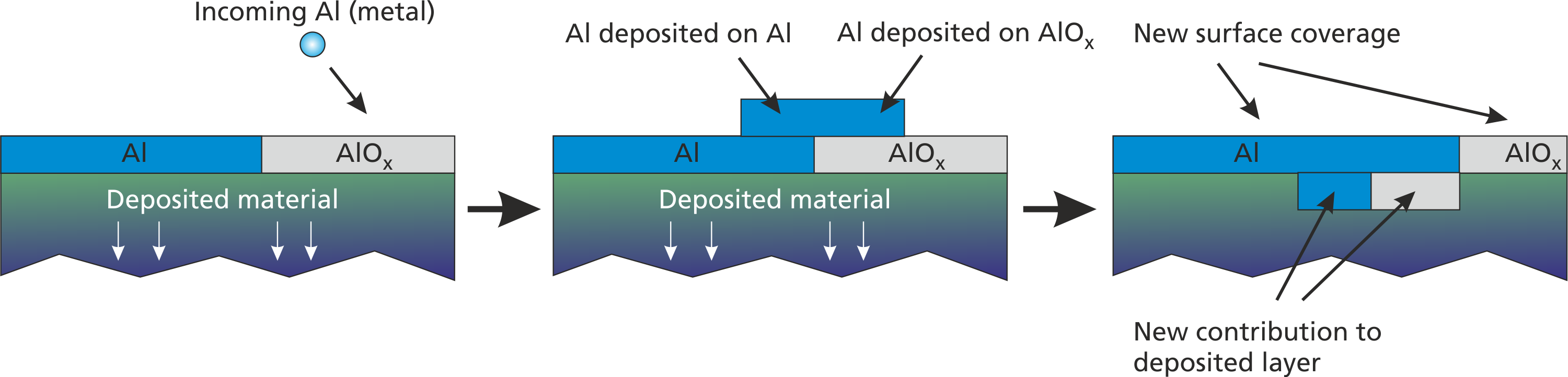
For this cover deposition, a special command can be used:
add_cover_deposition("species", amount, probability,
                     "deposition_material",
                     ["rp1", "rp2", ...], [n1, n2, ...]);
Here, the deposition_material parameter specifies, which material is deposited on top of all possible surface materials. In the reactive AlOx example, the following definitions are equivalent:
add_surface_deposition("Al", 1, 1.0, "Al", "Al", "Al", 1, [], []);
add_surface_deposition("Al", 1, 1.0, "AlOx", "Al", "AlOx", 1, [], []);
… and …
add_cover_deposition("Al", 1, 1.0, "Al", [], []);2.1.7.5 Implantation
A third deposition mechanism performs deposition by implantation, i. e. without modifying the state of the top surface layer:
add_implantation("species", amount, probability,
                 "deposition_material",
                 ["rp1", "rp2", ...], [n1, n2, ...]);
Here, the deposited_material is implanted into the layer through the top surface layer and without altering the surface coverage configuration. A visualization of such process in given in Fig. 2.5.
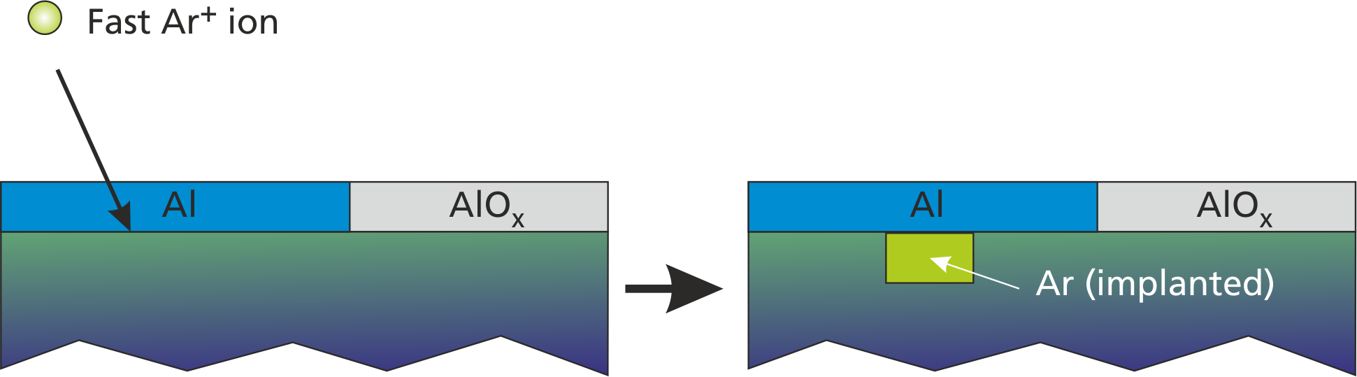
The accordant command for introducing Ar implantation by fast Ar+ bombardment with 20% probability is
add_implantation("Arplus", 1, 0.2, "Ar", ["e"], [0.05]);
set_emission_energy("e", 0, 10, 1.0);
Here, additionally a low-energy secondary electron (E=0..10 eV) can be emitted with 5% probability during such process.
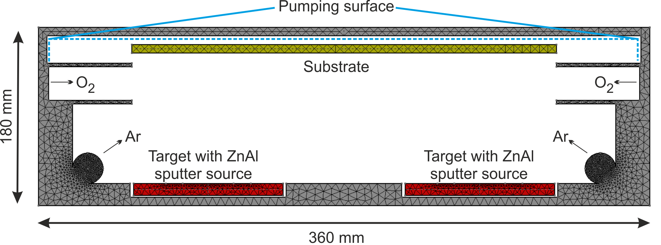
2.1.7.6 Example for a surface chemistry model for reactive ZnO:Al deposition
In this example, the reactive deposition of doped ZnO:Al layers is analyzed (Pflug et al. 2015). Especially the doping efficiency of the Al dopant is investigated. For this purpose, a simplified DSMC reactor model consisting of two Zn:Al sputter sources, an Ar gas inlet, an O2 gas inlet as well as a substrate is considered (see Fig. 2.6).
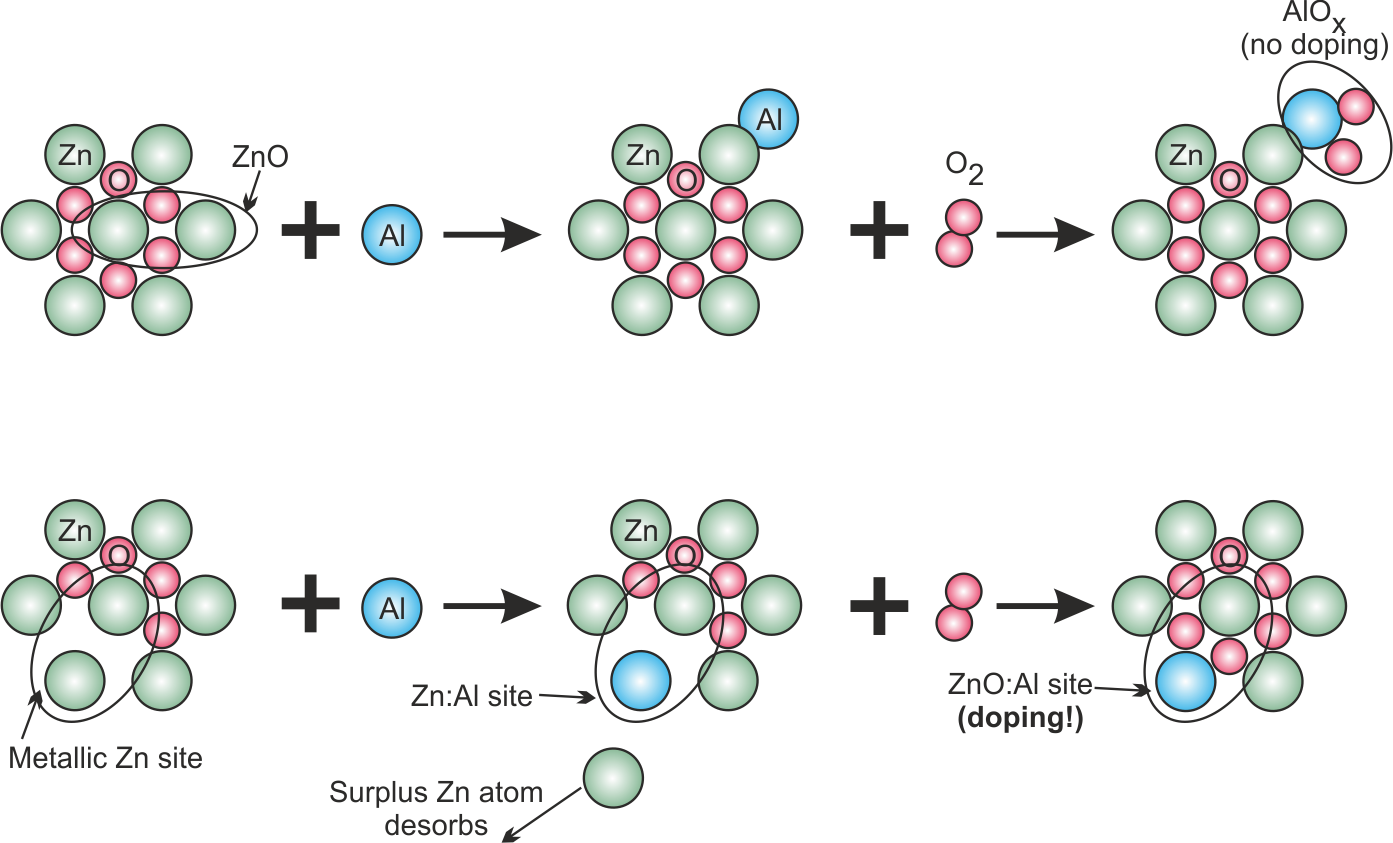
For the inclusion of Al into the ZnO, the following hypothetical model is constructed (see Fig. 2.7):
- On the one hand, metallic Zn coated on the substrate has a low binding energy (in fact, metallic Zn has a high vapor pressure). Thus, it should be rather easy for an incoming Al atom to replace one Zn atom on the surface thereby creating a Zn:Al mixed site.
- We assume that oxidation of a Zn:Al mixed site leads to a ZnO:AlO site, where the Al atom can act as dopant
- If the substrate is covered by ZnO on the other hand, the binding energy is rather high. Thus, an incoming Al atom is not able to replace a Zn atom and is rather being deposited as a separate Al site.
- The oxidation of separate Al sites leads to formation of separated, insulating AlOx clusters, which do not contribute to the doping process.
With four gas species "Ar", "O2", "Zn", "Al" the above described growth model can be implemented via the wall reaction model as shown in the following:
  # Initialize six possible surface material compounds:
  add_material("Zn2",      2e17);
  add_material("Al2",      2e17);
  add_material("Zn2O2",    2e17);
  add_material("ZnAl",     2e17);
  add_material("ZnOAlO",   2e17);
  add_material("Al2O3",    2e17);
  set_initial_coverage("Zn2",      0.5);
  set_initial_coverage("Zn2O2",    0.5);

  # Oxidation of Zn (gettering coefficient 50%)
  add_surface_reaction("O2",  1, 1, 0.5, "Zn2", "Zn2O2", [], []);

  # Exchange reaction Al (gas) + Zn2 (solid) --> ZnAl (solid) + Zn (gas)
  add_surface_reaction("Al",  1, 1, 1.0, "Zn2", "ZnAl", ["Zn"], [1]);

  # Exchange reaction Zn (gas) + Al2 (solid) --> ZnAl (solid) + Al (gas)
  add_surface_reaction("Zn",  1, 1, 1.0, "Al2", "ZnAl", ["Al"], [1]);

  # This is the insulating  species (gettering coefficient 70%)
  add_surface_reaction("O2", 1, 1.5, 0.7, "Al2", "Al2O3", [], []);

  # This is the doped oxide species (gettering coefficient 70%)
  add_surface_reaction("O2", 1, 1, 0.7, "ZnAl", "ZnOAlO", [], []);

  # Film growth by Zn or Al covering deposition
  add_cover_deposition("Zn", 2, 1, "Zn2", [], []);
  add_cover_deposition("Al", 2, 1, "Al2", [], []);
2.1.8 Particle sources depending on surface state
Particle sources may change their behavior depending on their surface coverage. Two different options are currently implemented as shown in the following.
2.1.8.1 Sputtering sources with given ion flux
A sputtering source with a given ion flux is given by the command
add_surface_emission("material", ion_flux,
                     ["rp_1", "rp_2", ...], [yield_1, yield_2, ...]);
Parameters are as in the following:
- material: Material phase in the surface layer. For different surface materials different sputtering processes can be defined.
- ion_flux: The effective ion flux is given in sccm.
- [“rp_1,” “rp_2,” …]: list of gaseous reaction products
- [yield_1, yield_2, …]: list of partial yields of the gaseous reaction products
The sputtering yield of a gasous reaction product is the product of the reaction probability and its partial yield. As an example, the surface chemistry and sputtering source for the reactive TiOx process is given:
# Specification of surface material phases and initial coverage:
add_material("Ti_metallic", 9e18);
add_material("TiO2",        9e18);
set_initial_coverage("TiO2", 0.9);

# Surface reactions:
add_surface_reaction("O2", 1, 1, 1.0, "Ti_metallic", "TiO2", [], []);
add_cover_deposition("Ti", 1, 1, "Ti_metallic", [], []);

# Sputtering source:
add_surface_emission("Ti_metallic", ion_flux_sccm, ["Ti"], [0.5]);
set_emission_thompson("Ti", 4.89, 1.0, 400, 40);
add_surface_emission("TiO2", ion_flux_sccm, ["Ti", "O2"], [0.05, 0.05]);
set_emission_thompson("Ti", 6.0, 1.0, 400, 40);
set_emission_thompson("O2", 6.0, 1.0, 400, 40);
In the above example, sputtering of metallic Ti and oxidized TiO2 is handled separately. The sputtering yield of TiO2 is by factor of 10 lower compared to metallic Ti. The energy distributions of the sputtered gaseous species are to be specified afterwards for each case.
Note: When sputtering the surface layer, it is being replaced by the material beneath the surface layer:
- If there is deposition on the sputtering surface, the replaced surface fractions are according to the stoichiometry of the material in the deposition layer.
- If there is no deposited material beneath the surface layer, the replacement material will be the material which is firstly defined in the deposition chemistry (i.e. Ti_metallic in the above example).
2.1.8.2 Thermal desorption of coated material
If surfaces are coated with materials with high vapour pressure, there is the possibility of thermal desorption of that material. For this purpose, a desorption source is implemented. It can be declared via the syntax
add_desorption("species", pressure, "material", amount);The parameters are as follows:
- species: The species, which is to be emitted from the wall into the gas phase
- pressure: The vapor pressure in Pa. The vapor pressure generally depends on the wall temperature. For many materials, the vapor pressure curve as a function of temperature is available in literature (Alcock, Itkin, and Horrigan 1984).
- material: The associated wall material.
- amount: The number of gas molecules needed to form a bond site of the wall material
If the surface material does not completely desorb but leaves behind some remainder, modified command is available:
add_desorption_r("species", pressure, "material",
                 amount_gas_species, "remainder", amount_remainder);
Here, we have the following parameters:
- species: The species, which is to be emitted from the wall into the gas phase
- pressure: The vapor pressure in Pa.
- material: The associated wall material.
- amount_gas_species: The number of gas molecules needed to form a bond site of the wall material.
- remainder: The wall material which is left behind by the desorption process.
- amount_remainder: The number of wall sites of the remaining material created by the desorption process.
Example: If we have a metallic ZnAl mixed site and assume that only Zn can desorp and leave behind a half Al2 site, the command would look like follows:
add_desorption_r("Zn", vapor_pressure, "ZnAl", 1, "Al2", 0.5);2.1.9 Electric boundary conditions in plasma simulation
In PIC-MC plasma simulations, mesh objects act as electrodes which are either conductive or dielectric (= insulating). Conductive electrodes can be either put on a fixed potential, they can be floating or they can have a built-in potential relative to another electrode. This behaviour can be specified by the parameters epsr, vf, vf_coupling as summarized in the following table.
Note 1: Electrodes need to be closed 3D objects in the mesh geometry. If you need particle sources which are part of an electrode, this is currently not supported (in DSMC simulation, it is possible to have source surfaces which are only part of a complete 3D object). A workaround is to use membranes as particle sources, since membranes do not act as electrodes in plasma simulation.
| Case | epsr | vf | vf_coupling |
|---|---|---|---|
| Dielectric domain (insulator) | |||
| Conductive floating potential | |||
| Fixed voltage | |||
| Voltage with self bias | |||
| Relative voltage |
A couple of pre-defined parameters and functions can be used in the voltage function string vf. RVM comes with a set of mathematical functions like sin, cos, atan,...,etc. Additionally the keywords TIME, VP and PI can be used within in the mathematical expression:
- TIME - The current simulation time, i.e. time step x current iteration.
- PI - You guessed it, pi (3.14159265).
- VP - Internally controlled voltage to meet aimed power dissipation
PSOLL, which could be a time-dependent function or absolute an value.
The use of the electric boundary conditions in typical scenarios is shown in the following pages within three examples.
Example 1: System of three walls, Target, Chamber and dielectric Substrate
block BORDER_TYPES: {
  Border Target: {
    icodec =  1;
    type   = "wall";
    T      = PAR.T0;
    reactions: {
      add_plain_reaction("Arplus", 1, 1, ["Ar", "e"],
                         [1, PAR.SECONDARY_ELECTRON_YIELD]);
      set_emission_energy("e", 0, 5, 1);
      add_absorption("e", 0.5);   # 50% electron reflection
    };
    vf = "-VP";  # Negative voltage amplitude for DC operation
  };

  Border Chamber: {
    icodec =  2;
    type   = "wall";
    T      = PAR.T0;
    reactions: {
      # We neglect secondary electrons at chamber and substrate surface
      add_absorption("Arplus", 1);
      add_absorption("e", 0.5);
    };
    vf = "0"; # Chamber wall grounded and on anode potential
  };

  Border Substrate: {
    icodec =  3;
    type   = "wall";
    T      = PAR.T0;
    reactions: {
      add_absorption("Arplus", 1);
      add_absorption("e", 0.5);
    };
    # Dielectric constant of glass
    epsr = 6.0;

    # vf must be commented out or deleted for a dielectric material.
    # vf = "";
  };
};
Example 2: The same system with floating conductive Substrate and with radio-frequency sputtering
block BORDER_TYPES: {
  Border Target: {
    icodec =  1;
    type   = "wall";
    T      = PAR.T0;
    reactions: {
      add_plain_reaction("Arplus", 1, 1, ["Ar", "e"],
                         [1, PAR.SECONDARY_ELECTRON_YIELD]);
      set_emission_energy("e", 0, 5, 1);
      add_absorption("e", 0.5); # 50% electron reflection
    };
    # RF (13.56 MHz) voltage
    vf = "VP*cos(2*PI*13.56e6*TIME)";

    # Indicates that this electrode has a self-bias
    vf_coupling = "Target";
  };

  Border Chamber: {
    icodec =  2;
    type   = "wall";
    T      = PAR.T0;
    reactions: {
      # We neglect secondary electrons at chamber and substrate surface
      add_absorption("Arplus", 1);
      add_absorption("e", 0.5);
    };
    vf = "0"; # Chamber wall grounded and on anode potential
  };

  Border Substrate: {
    icodec =  3;
    type   = "wall";
    T      = PAR.T0;
    reactions: {
      add_absorption("Arplus", 1);
      add_absorption("e", 0.5);
    };
    # Both, epsr and vf, must be commented out or
    # deleted for a floating conductor
  };
};
Example 3: Two targets Target_1, Target_2 acting as bipolar electrodes with 100 kHZ
block BORDER_TYPES: {
  Border Target_1: { # floating conductor, i.e. no vf, epsr, vf_coupling!
    icodec =  1;
    type   = "wall";
    T      = PAR.T0;
    reactions: {
      add_plain_reaction("Arplus", 1, 1, ["Ar", "e"],
                         [1, PAR.SECONDARY_ELECTRON_YIELD]);
      set_emission_energy("e", 0, 5, 1);
      add_absorption("e", 0.5);  # 50% electron reflection
    };
  };

  Border Target_2: {
    icodec =  4;
    type   = "wall";
    T      = PAR.T0;
    reactions: {
      add_plain_reaction("Arplus", 1, 1, ["Ar", "e"],
                         [1, PAR.SECONDARY_ELECTRON_YIELD]);
      set_emission_energy("e", 0, 5, 1);
      add_absorption("e", 0.5);   # 50% electron reflection
    };

    vf = "VP*cos(2*PI*100e3*TIME)";  # HF voltage signal
    vf_coupling = "Target_1";        # Counter electrode
  };

  Border Chamber: {
    icodec =  2;
    type   = "wall";
    T      = PAR.T0;
    reactions: {
      # We neglect secondary electrons at chamber and substrate surface
      add_absorption("Arplus", 1);
      add_absorption("e", 0.5);
    };
    vf = "0";  # Chamber wall grounded and on anode potential
  };

  Border Substrate: { # floating conductor, i.e. no vf, epsr, vf_coupling!
    icodec =  3;
    type   = "wall";
    T      = PAR.T0;
    reactions: {
      add_absorption("Arplus", 1);
      add_absorption("e", 0.5);
    };
  };
};
2.1.10 Sampling of energy and angular distribution
Each particle hitting a surface can be recorded within an energy or angular histogram vector. This functionality is applicable for walls as well as for membranes.
All histograms are taken per physical surface. Important: For membranes, the histogram is only taken for particles hitting the side, where the normal vector points out. This is useful if e. g. multiple histograms shall be taken for a large physical surface at different areas: In this case it is possible to use several transparent membranes placed close to the surface at the desired locations. Since particles hitting the surface can be diffusely reflected, it would be misleading if the reflected particles are also sampled by the membranes.
The involved commands for generating histograms must be written within the wall description blocks (see begin of this chapter (sec:prep_wall_model?)) and are listed in the following.
2.1.10.1 Energy histogram
The following command specifies a histogram for the electron energy distribution function, where the angular distribution is considered as isotropic.
add_energy_histogram("species", E0, E1, nE);Parameters are:
- species: The gas species which shall be recorded
- E0, E1: Energy interval of interest
- nE: Number of histogram points within \([E_0, \ldots E_1]\)
2.1.10.2 Angular histogram
The following command specifies a histogram for the angular distribution function only, i.e. not considering the energy distribution function.
add_angular_histogram("species", nTheta, nPhi, vx, vy, vz);Parameters are:
- species: The gas species which shall be recorded
- nTheta: The number of polar angle intervals (\(\theta\in [0,90]\))
- nPhi: The number of azimuth angle intervals (\(\phi\in [0,360]\))
- vx, vy, vz: A vector defining the direction where the azimuthal angle \(\phi\) shall be defined as zero5
2.1.10.3 Combined histogram
It is possible to use the above commands for energy and angular histogram, separately, which would yield two statistically independent distribution functions for energy and angle. Since energy and angular distribution can be correlated, it is also possible to generate a combined energy and angular distribution.
add_histogram("species", nTheta, nPhi, E0, E1, nE, vx, vy, vz);The parameters have the same meaning as in the single functions described above. In fact, this function is always internally called (also by add_energy_histogram and add_angular_histogram with a reduced parameter set). For a combined histogram please take care of the total number of histogram points (nThetanPhinE): If that number is very large, a very long time averaging interval will be needed to obtain useful statistics.
The resulting files in the output directory have the filenames histogram_<number>_<Surface>_<Species>_<Timestamp>.txt, e. g. histogram_1_Substrate_Ti_60.00ms.txt6.
The output format is just four columns with numbers:
- Energy [eV]
- Theta [°]
- Phi [°]
- Sampled histogram intensity
When making polar contour plots of the angular distribution, remember to adjust the intensity:
Intensity / sin(theta*pi/180)The reason for this is the integration in spherical coordinates, where the differential element is: \(\sin(\theta)d\theta d\phi\).
2.1.10.4 Histogram array
It is possible to divide a physical surface into an array of histograms. This only works for single plane surfaces by using the following command:
add_histogram_array("species", nTheta, nPhi,
                    E0, E1, nE, nX, nY,
                    x1, y1, z1, x2, y2, z2, x3, y3, z3);
Parameters are:
- species: The gas species which shall be recorded
- nTheta: The number of polar angle intervals (\(\theta\in [0,90]\))
- nPhi: The number of azimuth angle intervals (\(\phi\in [0,360]\)))
- E0, E1: Energy interval of interest
- nE: Number of histogram points within \([E_0, \ldots E_1]\)
- nX, nY: Number of histograms in x- and y-direction
- x1, y1, z1: First anchor point P1 of the histogram plane
- x2, y2, z2: Seconds anchor point P2, defines together with P1 the x-direction
- x3, y3, z3: Third anchor point P3, defines together with P1 the y-direction
The point coordinates should be given in mesh units. In the resulting file instead of a single intensity column, there are $n_X n_Y$ columns with the order \(I_{00}, I_{10}, I_{20}, \ldots I_{n_X-1\,nY-1}\). If \(i_x, i_y\) are the indices of the X and Y partition and \(i_c\) is the column number, the conversion rules are
\[\begin{aligned} i_c & = i_x + n_X i_y \in [0,\ldots \left(n_X n_Y\right)-1]\nonumber\\ i_x & = i_c\, \textrm{mod}\, n_X \in [0,\ldots n_X-1] \nonumber \\ i_y & = \lfloor i_c/n_X\rfloor \in [0,\ldots n_Y-1] \nonumber \end{aligned}\]
Warning: Please take care not to use too many histogram slots / histogram segments as this could easily lead to memory overflow. If a simulation run with large histogram arrays is crashing on startup, please check the memory consumption on the compute nodes and consider using a fewer number of slots / histogram segments.
Besides the general function, there are also an energy (add_energy_histogram_array) and angular (add_angular_histogram_array) only function. Their parameters are a subsection of the more general command above, the syntax is as follows:
add_energy_histogram_array(species, E0, E1, nE, nx, ny,
                           x1, y1, z1, x2, y2, z2, x3, y3, z3);
add_angular_histogram_array(species, nTheta, nPhi, nx, ny,
                           x1, y1, z1, x2, y2, z2, x3, y3, z3);
References
e.g. if a modified mesh file with different physical surface numbers shall be used with a given parameter file, this process is error-prone, you need to be careful↩︎
If the neutral density of Ar is very high with respect to ions and electrons, it might make sense to define a special species such as
ArFastin order to distinguish the fast reflected neutrals from the background gas↩︎average value↩︎
i. e. “AlOx” stands for a “half Al2O3 molecule”↩︎
This is mandatory, since otherwise the tangential vectors needed to compute the azimuthal angle are undefined↩︎
The 'number' is required since different histogram types are possible for the same species and surface, which would lead to the same filename otherwise↩︎