5.1.1 Geometric model

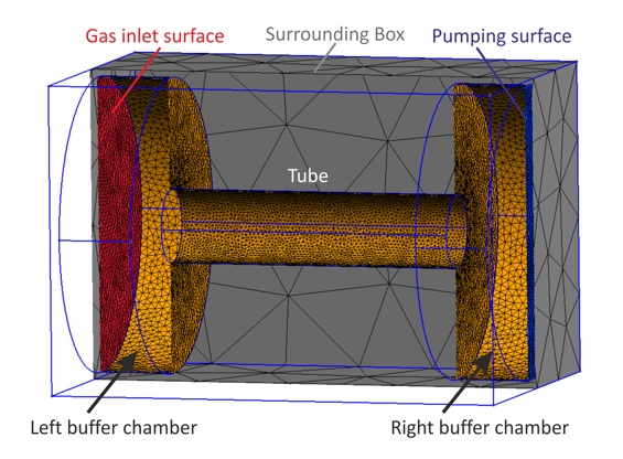
In this example, we analyze the gas flow through a cylindrical tube. The geometric model as shown in Fig. 5.1 contains the following elements:

• The cylindrical tube
• A buffer chamber at the left side of the tube for simulation of the gas inflow
• A buffer chamber at the right side of the tube for simulation of the gas outflow
• A gas inlet surface within the left buffer chamber
• A pumping surface within the right buffer chamber
• A box surrounding all above mentioned elements

5.1.2 General considerations about geometries for gas flow simulation

In order to create such a model, we use the open source meshing and postprocessing tool GMSH (Geuzaine and Remacle (2009)). There are two possible ways of creating geometric model with GMSH: Either the model can be created manually by GMSH's own interactive mode and scripting language, or an IGS file (or STEP or other formats) originating from a CAD system can be imported. For our example, we use the manual way in order to point out the most relevant parts of a geometric model definition. Before starting to create the model, the following points are to be considered:

• At first, it is important to mention that we will create a surface mesh rather than a volume mesh. Within the DSMC/PIC-MC code, the surface mesh will be used to track collisions between particles and chamber walls, while collisions between the particles will be treated within a cartesian volume grid, which is created independently from the surface mesh model.
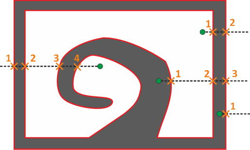
• Second, each wall has to be represented by at least two surfaces (for front and back side). This is important for determining, whether a given point lies within a wall or within the free space. The algorithm which decides about that is pointed out in Fig. 5.2. From a given point in space, a virtual line is drawn along X axis¹, and the number of intersections between this line and any mesh surface is counted. For an even number of intersections, the point is considered to be within the gas flow volume, while for an uneven number of intersections, the point is considered to be within a solid wall.

5.1.3 Definition of geometric points

Before creating the model, we need to think about some conventions about the coordinates, orientation, units etc. In this example, we stick to the following conventions:

• All length units are in mm
• The tube is oriented along X axis
• The coordinate origin (0,0,0) is located at the left end of the tube, centralized within the circular cross section

A geometric model always consists of points, lines, and surfaces. First, the geometric points have to be defined, second, the points are connected with lines and finally, surfaces are defined by line loops. The definition of point coordinates is done in GMSH’s scripting engine as shown in the following.

First, some global variables are defined in the file header

LC = 10;  // characterictic mesh size

L_TUBE = 400;
R_TUBE =  50;

L_BUFFER = 100;
R_BUFFER = 200;

WALL = 10;

Next is the definition of inlet and outlet points for the cylindrical tube

// Tube orientation along x axis

// Center point at left tube edge
Point(101) = {0, 0, 0, LC};  

// Four points on tube radius separated by 90 degree
Point(102) = {0,  R_TUBE, 0,       LC};
Point(103) = {0,  0,      R_TUBE,  LC};
Point(104) = {0, -R_TUBE, 0,       LC};
Point(105) = {0,  0,      -R_TUBE, LC};

// The same is repeated for the right tube edge
Point(106) = {L_TUBE,  0,      0,       LC};  
Point(107) = {L_TUBE,  R_TUBE, 0,       LC};
Point(108) = {L_TUBE,  0,      R_TUBE,  LC};
Point(109) = {L_TUBE, -R_TUBE, 0,       LC};
Point(110) = {L_TUBE,  0,      -R_TUBE, LC};

Adjacent to both tube ends are located two larger cylinders which act as buffer chambers for the gas inlet and for the pumping.

// Additionally, we need buffer chambers at 
// left and right side of tube
// Left buffer chamber:
Point(201) = {-L_BUFFER,  0,         0, LC};
Point(202) = {-L_BUFFER,  R_BUFFER,  0, LC};
Point(203) = {-L_BUFFER,  0,         R_BUFFER, LC};
Point(204) = {-L_BUFFER, -R_BUFFER,  0, LC};
Point(205) = {-L_BUFFER,  0,        -R_BUFFER, LC};
Point(206) = {0,  R_BUFFER,  0, LC};
Point(207) = {0,  0,         R_BUFFER, LC};
Point(208) = {0, -R_BUFFER,  0, LC};
Point(209) = {0,  0,        -R_BUFFER, LC};

// Right buffer chamber:
Point(302) = {L_TUBE,           R_BUFFER,  0, LC};
Point(303) = {L_TUBE,           0,         R_BUFFER, LC};
Point(304) = {L_TUBE,          -R_BUFFER,  0, LC};
Point(305) = {L_TUBE,           0,        -R_BUFFER, LC};
Point(301) = {L_TUBE+L_BUFFER,  0,         0, LC};
Point(306) = {L_TUBE+L_BUFFER,  R_BUFFER,  0, LC};
Point(307) = {L_TUBE+L_BUFFER,  0,         R_BUFFER, LC};
Point(308) = {L_TUBE+L_BUFFER, -R_BUFFER,  0, LC};
Point(309) = {L_TUBE+L_BUFFER,  0,        -R_BUFFER, LC};

Finally, the whole arrangement is surrounded by an outer wall, which is shaped as a rectangular box.

// Bounding box around the whole setup

x0 = -L_BUFFER-WALL;
x1 =  L_BUFFER+L_TUBE+WALL;
y0 = -R_BUFFER-WALL;
y1 = R_BUFFER+WALL;
z0 = -R_BUFFER-WALL;
z1 = R_BUFFER+WALL;

Point(401) = {x0, y0, z0, LC*5};
Point(402) = {x1, y0, z0, LC*5};
Point(403) = {x0, y1, z0, LC*5};
Point(404) = {x1, y1, z0, LC*5};
Point(405) = {x0, y0, z1, LC*5};
Point(406) = {x1, y0, z1, LC*5};
Point(407) = {x0, y1, z1, LC*5};
Point(408) = {x1, y1, z1, LC*5};

A few comments on this code are given in the following:

• In the first line, a variable LC is defined, which is subsequently used as fourth argument for each Point. This is a characteristic length and defines the average mesh size around the points.
• Further characteristics dimensions such as the tube length (L_TUBE), its radius etc. are also defined as variables, which are subsequently being used in the point coordinates. This simplifies to create variations of the geometric model with different tube lengths etc. later on.
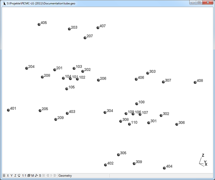
• The syntax of a point definition in GMSH is Point(number)={x, y, z, lc}; The point number must be unique within the whole GMSH model. It is not required that the set of numbers is continuous. It is convenient to assign the same major number to points which belong to a certain part of the geometry, e.
  7. 1XX for the tube, 2XX for the left buffer chamber etc.
• Wherever a coordinate is required in GMSH it is possible to make use of a built-in formula parser.
• If you copy the above script into an ASCII file (named e. g. 'tube3d.geo') and open this file with GMSH, you will get a picture similar as in Fig. 5.3.

5.1.4 Definition of straight lines and circle arcs

The next step is to connect all points with straight or circular lines. This can be either done by further script commands or by using GMSH interactively. We will follow the interactive way. First, use the GMSH menu sequence shown in Fig. 5.4 in order to select "circle arcs".

A circle arc is now created by clicking on three points subsequently: (i) A point on the circle as start point, (ii) the center of the circle and (iii) another point on the circle as end point. The left circular entrance of the tube is e. g. defined by clicking on points no. 102-->101-->103; 103-->101-->104; 104-->101-->105; 105-->101-->102. The right circular entrance of the tube is defined analogously (107-->106-->108; 108-->106-->109; 109-->106-->110; 110-->106-->107).

After having defined both circular surfaces, please click on "Straight line" in the GMSH menu and connect the following points: 102-->107; 103-->108; 104-->109; 105-->110. The interactive GMSH graph should now look as in Fig. 5.5.

While interactively defining lines between the points, GMSH automatically appends accordant script lines to the geometry script. If you look at the ASCII file tube2d.geo, you will find the following lines automatically appended at its end³.

Circle(1) = {102, 101, 103};
Circle(2) = {103, 101, 104};
Circle(3) = {104, 101, 105};
Circle(4) = {105, 101, 102};
Circle(5) = {108, 106, 109};
Circle(6) = {109, 106, 110};
Circle(7) = {110, 106, 107};
Circle(8) = {107, 106, 108};
Line(9) = {102, 107};
Line(10) = {103, 108};
Line(11) = {104, 109};
Line(12) = {105, 110};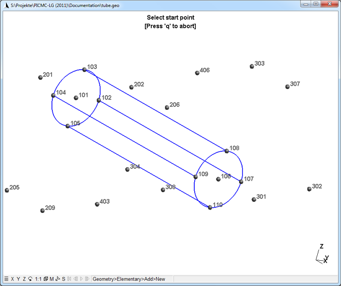

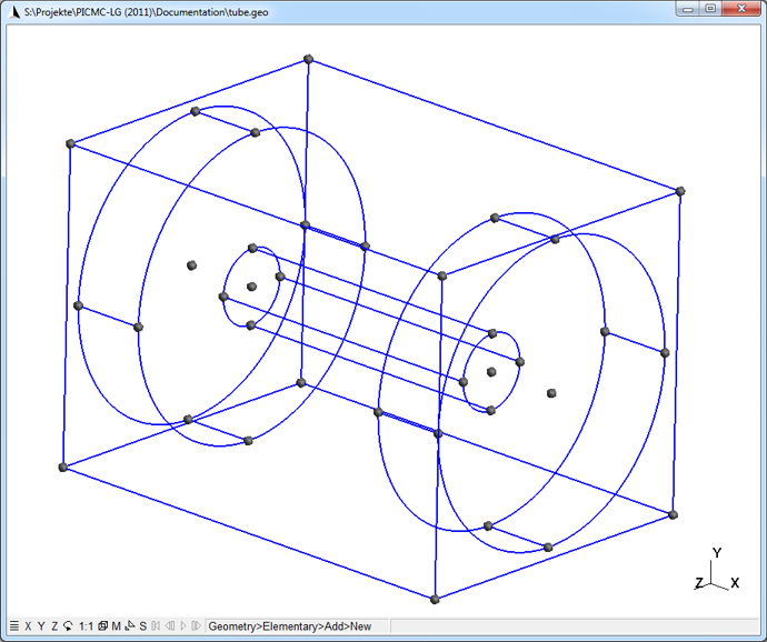
By continuing in the same manner, all other circle arcs and straight lines are to be defined. At the end, each point will be part of at least one line or circle arc, and the geometry will look like in Fig. 5.6. At this stage, please press the "q" button in order to leave the line selection mode. For your convenience, a zipped file of this stage (i. e. all points and lines but no surfaces) is provided for download.

5.1.5 Definition of ruled and plain surfaces

The next step will be to define the surfaces. In this case, we have to distinguish between

• Plane surfaces and
• Ruled surfaces.

Ruled surfaces are required for the cylindrical walls of the tube and buffer chambers. By the straight lines, the cyclindrical wall of the tube is divided into four parts. Each part has to be selected, individually.

In order to start building surfaces, please select the entry "Ruled Surface" within the GMSH menu shown in Fig. 5.4. Subsequently, select one of the four possible line loops on the cylindrical wall as shown in Fig. 5.7. This is accomplished by clicking onto lines rather than onto points. If you mis-clicked a line, pressing on "u" will undo the last selection. When all appropriate lines are highlighted as shown in Fig. 5.7, press "e" in order to confirm the selection.

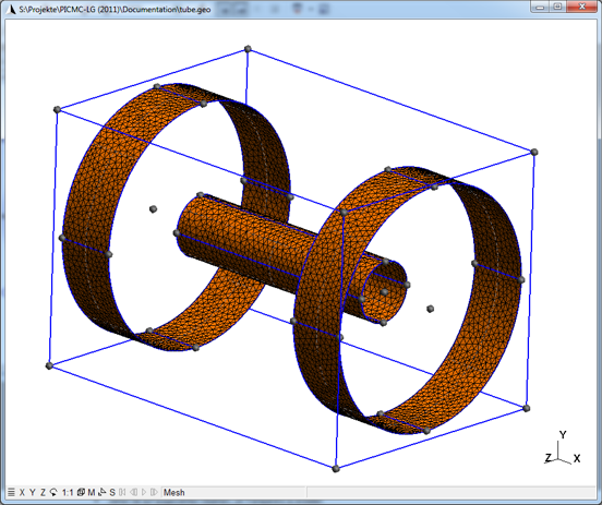
This process has to be repeated for all four partial surfaces of the tube as well as of both buffer chambers. In total, twelfe "Ruled Surfaces" are required. After having defined all ruled surfaces, please press "2" in order to obtain a two-dimensional surface mesh, which will yield a picture similar as in Fig. 5.8.

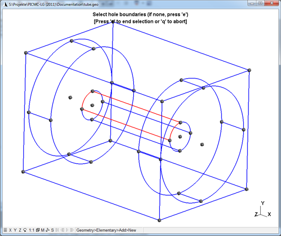
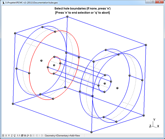
Finally, the remaining plane surfaces should be defined. These are the plane surfaces of the surrounding box as well as front and back surfaces of the buffer chambers. Important: There should be no surfaces defined for both tube entrances, since otherwise the gas flow will be blocked. Instead, the adjacent surface of the buffer chamber is to be defined with the tube entrance as hole boundary. This is accomplished by first selecting the outer line loop of the large buffer chamber and then selecting the inner line loop of the tube entrance and finally pressing on "e". Fig. 9 shows a possible way of doing this. Please proceed with all remaining plain surfaces in order to come to the final step of defining physical surface groups. The attached ZIP file contains the geometry model with all surfaces but without any physical surface group.

5.1.6 Physical surface groups

The surfaces of our tube model are supposed to have different physical functions. While most of the surfaces are just acting as walls, where particles are being diffusively reflected, there is also an inlet and a pumping surface. Thus, we expect to define three different physical surface groups:

• Wall --> All surfaces except from inlet and outlet surfaces
• Inlet --> The left surface of the left buffer chamber
• Pump --> The right surface of the right buffer chamber

In order to select physical surface groups in GMSH, please use the menu sequence as shown in Fig. 5.10.

An appropriate strategy is to first select all surfaces in the model in order to form the physical surface group for "Wall". Afterwards, the "Inlet" and the "Pumping" surface should be individually selected. In order to select all surfaces, the following steps are required:

• With the center mousebutton, select an appropriate zoom in the GMSH window, where the whole geometry becomes visible.
• Hold down the "Ctrl" key and click once at a location in the upper left from the geometry.
• Release the "Ctrl" key and move the mouse cursor to the lower right. A dotted frame will appear, when this frame encloses the whole geometry, click on the mouse button the second time (see also Fig. 5.11 below).
• All surfaces will appear in red now, if this is the case, press "e" to confirm the selection.

Afterwards, please select the left plane surface of the left buffer chamber as well as the right surface of the right buffer chamber individually. After having completed the physical surface selection, GMSH has added three more lines to the geometry script, which look similar as follows:

Physical Surface(95) = {60, 92, 62, 52, 54, 72, 77, 86, 50, 58, 64, 56, 70, 75, 84, 88, 80, 66, 68, 82, 90, 94};
Physical Surface(96) = {77};
Physical Surface(97) = {82};

Here, we have to apply some changes manually. First, we would rather use strings than numbers in order to identify the physical surfaces. This can be done by replacing the numbers in round brackets by quoted strings as follows:

Physical Surface("Wall")  = {60, 92, 62, 52, 54, 72, 77, 86, 50, 58, 64, 56, 70, 75, 84, 88, 80, 66, 68, 82, 90, 94};
Physical Surface("Inlet") = {77};
Physical Surface("Pump")  = {82};

Since, we have selected all surfaces for the first physical surface group "Wall", the surfaces number 77 and 82 are now selected twice. These ambiguities must be removed; thus, the duplicate surface numbers (in our case 77 and 82) should be removed from the first physical surface group "Wall". As a final result, the last three lines of the GMSH file should now look as in the following:

Physical Surface("Wall")  = {60, 92, 62, 52, 54, 72, 86, 50, 58, 64, 56, 70, 75, 84, 88, 80, 66, 68, 90, 94};
Physical Surface("Inlet") = {77};
Physical Surface("Pump")  = {82};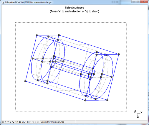

5.1.7 Final step: Saving the mesh file

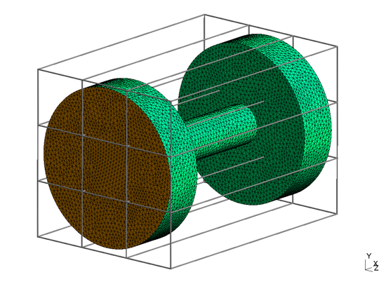
As a final step, a 2D surface mesh is created by pressing the "2" button. Afterwards, the mesh file can be saved by clicking on the "save" button of the GMSH main dialog. A complete version of the tube model can be found as "tube.geo" within this ZIP file.

5.2.1 Global control variables

The first section of the parameter file comprises some global variables for the simulation run and its runtime behavior. It should be edited like follows:

DT       = 1e-5;     # Time step width
TSIM     = 1.0;      # Total simulation time in seconds
TAVG     = 1;        # Time averaging mode (0 = off, 1 = on)
NPLOTS   = 10;       # Number of plots
NDUMPS   = 1;        # Number of particle data dumps
WORKMODE = 0;        # Work mode (0 = DSCM gasflow simuation, 
                     # 1 = PICMC plasma simulation, 
                     # 2 = electric field solver)
T0       = 300;      # Initial particle and border temperature [K]
PSOLL    = 1;        # Aimed power dissipation in Watt (plasma simulation only)
PSAMPLE  = 1e-7;     # Sampling time for power dissipation (plasma simulation only)
#VPMAX    = 1000;    # Maximum voltage for power control (default = 1000 volt)

5.2.2 Gas species and cell resolution

The next lines within the parameter file deal with the selection of gas species, their initial distribution and their statistical weight. In our test case, we will define a gas inlet operating with Argon at a pressure of 1.0 Pa and a pumping surface. This means, that the pressure will reach 1 Pa close to the gas inlet but will be significantly lower in the major part of the simulation volume. For Argon with a pressure of 1 Pa, the mean free path is approx. 6 mm, thus a cell dimension of about 0.5 mm would be required close to the gas inlet. Since we assume that the pressure in the tube will be significantly lower, we will start with a homogeneous pressure distribution of 0.5 Pa and use 1.0 cm as appropriate cell dimension.

In section ((sec:num_constraints_dsmc?)), for Argon with a pressure of 1.0 Pa, a cell dimension of 5 mm and a value of NREAL_Ar=3e12; is suggested, which leads to an average of 10 simulation particles per cell. To transfer this to the case with a pressure 0.5 Pa with 10 mm cell dimension, we need to keep in mind that NREAL_Ar scales reciprocally with the square of the pressure. Accordingly, the resulting value for NREAL_Ar is 1.2 x 10¹³. Thus, the lines within the parameter file should be edited as follows:

SPECIES  = ["Ar"];   # List of species strings
NREAL_Ar = 1.2e13;   # Default scale factor for Ar
P0_Ar    = 0.5;      # Default pressure of initial Ar distribution [Pa]

In the next lines of the parameter file, the desired output of the simulation run is specified:

NUMBER      = ["Ar"];
PRESSURE    = ["Ar"];
VELOCITY    = ["Ar"];
FIELD       = ["PHI"];

The next section of the parameter file deals with the bounding box, i.e. the simulation volume and its cell resolution. First, we have to define the length unit, which is used within the mesh file. Our geometry model uses mm as length unit, while the default setting in the parameter file is m. Thus, it is required to change the length UNIT to 0.001.

Next, the bounding box coordinates are shown within the array BB. It is possible to edit the BB array in order to restrict the simulation volume to a fraction of the mesh geometry, but we will use the full volume, here. The six numbers define two points in 3D with lower and upper coordinates. In our case, the bounding box spans between (-110,-210,-210)-->(510,210,210). Accordingly, the length of the bounding box is 62 cm in X direction and 42 cm in Y and Z direction. With the cell dimension of 10 mm as discussed above, we would like to have 62 cells along X direction and 42 cells in Y and Z direction, leading to a total of 109368 cells.

The cell resolution and segmentation of the simulation volume is defined in the arrays NX, NY, NZ. The segmentation is important with respect to parallel processing: Each segment of the simulation volume can be assigned to an indidividual CPU core. By this way, the number of segments limits the maximal number of parallel processes⁴. In the default settings, the simulation volume is divided into two segments along each axis, and each segment has a resolution of 10 grid cells. Given our model dimension, this seems not appropriate. For our purpose, we should change these lines to:

UNIT = 0.001;  # Unit of mesh geometry (1.0 [m], 0.001 [mm], 0.0254 [inch], ...) 
BB   = [-110, -210, -210, 510, 210, 210]; # Bounding box dimensions
NX   = [62];             # Cell resolution of subvolumes in x-direction
NY   = [14, 14, 14];     # Cell resolution of subvolumes in y-direction
NZ   = [14, 14, 14];     # Cell resolution of subvolumes in z-direction

By these settings, we divide the volume into three segments in Y and Z direction, while only one segment is used in X direction (see Fig. 5.12). The total number of segments is 3x3 = 9; thus, a maximal number of 9 parallel PIC-MC processes can be used for this simulation model. The numbers given for each segment denote the number of cells. In Y and Z direction we have have the 42 cells divided into three segments, i.e. 14 cells per segment, while in X direction we use 62 cells for one segment.

The selection of species, their statistical weights and the definition of the cell resolution is the most crucial part in the parameter file. The remaining steps are comparably easy.

5.2.3 Simulation domain - bounding box

The simulation domain has the shape of a cuboid, which may be divided into segments and sub-cells. It is required to specify the boundary conditions in case, if a simulation particle reaches a cuboid surface. Possible boundary conditions are outlet, specular and periodic. We have to distinguish between the following cases:

• In 3D models, usually the gas volume is contained into a closed mesh geometry. In this case, no particle should reach the cuboid boundary. If the mesh geometry is not rectangular, there may be particles originating from an initial homogeneous distribution, which are outside the gas volume. In all such cases the most appropriate boundary condition is outlet, i. e. a particle reaching the cuboid boundary will be deleted. The respective lines in the parameter file should look like follows:TYPE_x1 = "outlet"; TYPE_x2 = "outlet"; TYPE_y1 = "outlet"; TYPE_y2 = "outlet"; TYPE_z1 = "outlet"; TYPE_z2 = "outlet";{.C#}
• In some cases, there may be 3D models with a mirror symmetry plane. In such cases it is possible to reduce computation time by factor of two by placing one of the cuboid boundaries at the plane of symmetry. The appropriate boundary condition for such plane is specular, i. e. a particle hitting this surface will be specularly reflected. An example, where the cuboid boundary at lower Y coordinates defines a symmetry plane, is given as follows:TYPE_x1 = "outlet"; TYPE_x2 = "outlet"; TYPE_y1 = "specular"; TYPE_y2 = "outlet"; TYPE_z1 = "outlet"; TYPE_z2 = "outlet";{.C#}
• In 2D models, there are only mesh geometry elements for boundaries within e. g. the XY plane, while the geometry remains open in Z direction. In this case, both cuboid boundaries perpendicular to the Z axis should be either specular or periodic⁵.
• In 1D models, four of the six boundaries must be set on periodic or specular. This may look like follows:TYPE_x1 = "periodic"; TYPE_x2 = "periodic"; TYPE_y1 = "periodic"; TYPE_y2 = "periodic"; TYPE_z1 = "outlet"; TYPE_z2 = "outlet";{.C#}

5.2.4 Surface functions

Finally, the geometric mesh file is to be specified, and the functions of the respective physical surfaces must be defined. The specification of the mesh file's filename follows just after the boundary conditions of the bounding box:

# ==================================================
# Specify mesh files and boundary conditions
# Available border types are: "wall" and  "membrane"
# ==================================================
MESHFILE = "sample.msh"; # Name of mesh file for PICMC particle simulation
BEMMESH  = ""; # Name of mesh file for BEM b-Field solver

Here, only for MESHFILE a filename must be specified; BEMMESH is only used for computation of the magnetic field in PVD plasma simulation setups and can be left empty, here.

In the following parameter file section, the functions of the respective physical surfaces can be defined. A detailed description about the possibilities here is given in section (sec:prep_wall_model?). In our case we just need a particle source at surface Inlet and an absorption coefficient at surface Pump. The surface Wall is by default diffusely reflective at a temperature T0 and can be left unchanged. With these two modifications, the wall function definition block would look like follows:

block BORDER_TYPES: {
  Border Wall = {
    icodec =   1;        # Codec number from meshfile
    type = "wall";       # Alternative type: "membrane" 
    T = PAR.T0;          # Wall temperature
    #epsr        = 1.0;  # Rel. dielectric permittivity (insulator only)
    #vf          = "VP*cos(2*PI*13.56e6*TIME)"; # Voltage function (conductor only) 
    #vf_coupling = "";                          # Border name of counter electrode 
    reactions: {
      # Add reactions here - please check SIM-Wiki for available reaction schemes!
  };

  Border Inlet = {
    icodec =   2;        # Codec number from meshfile
    type = "wall";       # Alternative type: "membrane" 
    T = PAR.T0;          # Wall temperature
    # epsr = 1.0;        # Rel. dielectric permittivity (insulator only)
    # vf = "VP*cos(2*PI*13.56e6*TIME)"; # Voltage function (conductor only) 
    # vf_coupling = "";                 # Border name of counter electrode 
    reactions: {
      add_source("Ar", 1.0, "Pa");
    };
  };

  Border Pump = {
    icodec =   3;        # Codec number from meshfile
    type = "wall";       # Alternative type: "membrane" 
    T = PAR.T0;          # Wall temperature
    # epsr = 1.0;        # Rel. dielectric permittivity (insulator only)
    # vf = "VP*cos(2*PI*13.56e6*TIME)"; # Voltage function (conductor only) 
    # vf_coupling = "";                 # Border name of counter electrode 
    reactions: {
      add_absorption("Ar", 0.25);
    };
  };
};

The completed simulation case including GEO and PAR file can be downloaded here.