
DSMC and PICMC documentation
2024-09-20
4 Postprocessing
4.1 Data being generated during simulation runs
Each simulation case requires at least a geometric mesh file and a parameter file (e.g. simcase.par), where the simulation conditions, species, plasma-wall interaction etc. is contained. When the simulation is started, all resulting output data is written into a folder simcase/ which has the same name as the parameter file. The folder is automatically being created if it does not exist.
The output data generated during simulation can be divided into following categories:
| Type of data | Resolution | File Format | Output frequency |
|---|---|---|---|
| Information on gaseous species | Cell resolution | GMSH *.pos |
NPLOTS times |
| Wall absorption and desorption | Cell resolution | GMSH *.pos |
NPLOTS times |
| Wall state | Cell resolution | GMSH *.pos |
NPLOTS times |
| Surface data averaged by mesh elements | Mesh resolution | GMSH *.pos and ASCII *.txt |
NPLOTS times |
| Electromagnetic field data | Node resolution | GMSH *.pos |
NPLOTS times |
| Collision statistics | Averaged per segment | ASCII *.txt |
NPLOTS times |
| Logging of surface data | Integrated over physical surface | ASCII *.txt |
NCOUNTS log entries |
| Logging of potentials | Integrated over physical surface | ASCII *.txt |
NCOUNTS log entries |
| Cell structure and domain decomposition | – | GSMH *.pos and GMSH *.geo |
Upon startup |
| Used collision cross sections | – | Postscript or ASCII | Upon startup |
| Profiling data | Quad resolution | ASCII | Upon shutdown |
| Checkpoint of simulation data | – | Binary and ASCII | NDUMPS times and at the end or during shutdown |
| Dynamic script files | – | ASCII *.rd |
Upon startup |
4.1.1 Information stored in picmc cell structure
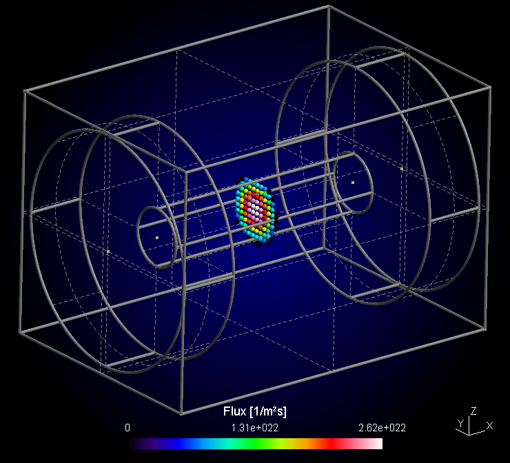
Most of the data volume is given as time- and particle averaged values within the cell structure. They are provided as POS files which can be viewed and further processed within GMSH.
These data can comprise information on gaseous species as well as on particle absorption and status of walls. Additionally, some data on particle absorption can be also given in the resolution of the surface mesh.
The time-averaging feature is activated by setting TAVG=1; at top of the parameter file. By setting TAVG=0; momentary snapshots are displayed instead, however in most cases they will be quite noisy or a very large number of particles has to be simulated to get reasonable statistics. Therefore, TAVG=1; is the default setting.
The number of time averages within the whole physical simulation time interval is defined in the variable NPLOTS at top of the parameter file. The selection of output data by species is defined via lists in the upper part of the parameter file.
The following lists for cell-oriented information are available:
- Information on gaseous species
NUMBER= Number of simulation particles per cellDENSITY= Density of simulation particles in physical units [1/m³]PRESSURE= Partial pressure in [Pa]TEMPERATURE= Translational kinetic temperature in [K]ENERGY= Mean particle energy in [eV]VELOCITY= Mean particle velocity in [m/s]. This is a vector plot for three components vx, vy, vz.
- Information on wall absorption and wall state
ABSORPTION= Particle absorption on walls in [1/m²s]DESORPTION= Particle desorption from walls in [1/m²s]COVERAGE= Surface coverage fraction of a wall material (between 0 and 1)DEPOSITION= Deposition rate of a wall material [nm/s]
- Information on fields
FIELD= Quantities concerning electromagnetic field computation
All of these data go into sub folders of the simulation data folder. This behaviour can be suppressed by setting SINGLE_PLOT_FOLDER=1; (which can be found in the bottom part of the parameter file).
The filename structure is <type>_<species>_<time>ms.pos, e.g. the Ti absorption after 50 ms will be stored in a file absorption/absorption_Ti_50.00ms.pos. These files can be opened and further processes in GMSH.
4.1.2 Collision statistics
The list COLLISION enables the plotting of collision statistics on quad resolution for every used cross section defined in the sigma.r file. By putting a species name in that list all reactions involving this species are written in a separate file including the energy threshold to identify the corresponding cross section. The weighted sum of all quads for a specific collision matches the total collision rate written in the collision.txt files present in the same folder.
4.1.3 Surface data allocated in triangular mesh elements
Additionally, with the list MESHDATA particle absorption information is given in the resolution of the surface mesh. The filename for mesh absorption data for Ti after 50 ms will be e.g. meshdata/meshdata_Ti_50.00ms.pos. These data files contain multiple plots:
- Absorption
- Desorption
- Mean energy of absorbed particles
- Mean angle of incidence \(\alpha\)
- Mean \(\cos(\alpha)\)
The POSITION list has to be handled with care. If you put a species in there, for all particles of that species the position and energy is plotted. This plot is used normally with a low number of particles, e.g. a high NREAL or individually distributed particles with the Init_Particles block. An example would be the movement of single electrons in the electromagnetic field.
The choice, which data to plot in cell or mesh resolution is done in the 3D data extraction section in the parameter file (see section (sec:par_plots?)). A typical choice setup may look as follows.
# ===================================================== #
# 3D data extraction                                    #
# Examples: NUMBER = ["Ar", "e"]; FIELD = ["PHI", "E"]; #
# ===================================================== #
NUMBER      = [];
DENSITY     = [];
PRESSURE    = ["Ar", "O2", "Ti"];
TEMPERATURE = [];
ENERGY      = [];
VELOCITY    = ["Ar", "O2", "Ti"];
COLLISION   = [];
ABSORPTION  = ["Ti"];
DESORPTION  = ["Ti"];
MESHDATA    = ["Ti"];
# POSITION plots can get very large, so handle with care!
POSITION    = [];
# "PHI" = electric potential, "PHI_MEAN" = time averaged electric potential,
# "E" = electric field
# "JICP" = source current density, "EICP" = current induced electric field,
# "BICP" = current induced magnetic field
FIELD       = [];

# For COVERAGE and DEPOSITION fill in required surface materials:
COVERAGE    = ["TiO2"];
DEPOSITION  = ["Ti_metal", "TiO2"];
With these settings, the pressure and velocity are plotted for three species, Ar, O2 and Ti, respectively. For Ti, additionally the absorption plot in cell resolution and absorption data in mesh resolution are generated. Finally, for wall materials TiO2 and Ti_metal the deposition rate is plotted together with the surface coverage fraction for TiO2.
4.1.4 Magnetic / electric field etc. on node structure
According to the "leap frog" algorithm used for the PIC-MC computation, the electric and magnetic field / potentials are computed per nodes rather than per cell. A cell "node" is one of the corner points of the cell, i.e. a rectangular cell has 8 nodes. The nodes are shared with the neighboring cells.
The file format is GMSH POS. However the node oriented data have one element more in each direction. This may cause issues in postprocessing together with cell oriented data. For an example, in the RIG-VM postprocessing routines (section (sec:ppp_rvm?)), cell oriented and node oriented data shall be processed in separate postprocessing objects.
The choice of electric / magnetic field and potential output can be done within the list FIELD in the parameter file. Possible choices are
- Capacitively coupled plasma (CCP)
"PHI"- Electric potential (momentary snapshot)"PHI_MEAN"- Electric potential, time averaged over the last time averaging period"E"- Electric field as gradient of PHI (momentary snapshot)
- Inductively coupled plasma (ICP)
"JC"- Primary current, i.e. coil surface current density"JE"- Secondary current, i.e. electron current (convection current) in plasma"EC"- Primary current induced electric field"EE"- Secondary current induced electric field"BC"- Magnetic field as curl of EC"BE"- Magnetic field as curl of EE
In the following example, the time averaged electric potential and the electric field are plotted:
FIELD = ["PHI_MEAN", "E"];4.1.5 Time dependent logging of averaged surface data
4.1.5.1 Particle balance at surfaces
During simulation, particles are absorbed and desorbed from surfaces and/or flowing through transparent membranes. In order to better track the current state of the simulation run, these processes are time averaged over physical surfaces and put into ASCII logfiles. The following log files are automatically created during simulation:
absorption_log.txt- Particle absorption on surfacesdesorption_log.txt- Particle desorption from surfacestransmission_log.txt- Particle flow through transparent membranespressure_log.txt- Kinetic pressure due to particle impingement on surfaces
By default, 100 log entries are created per simulation run. This number can be modified with the global variable NCOUNTS in the parameter file, e.g.
NCOUNTS = 1000;Each of the log files has the physical time in the first column. The other columns contain particle fluxes / pressures according to the headlines given in the file. The choice of columns is performed automatically according to the absorption / desorption mechanisms defined within the wall reactions.
Depending on if the particles are charged/neutral, absorption, desorption and transmission are given in [A] / [sccm]. Both units are proportional to the total number of particles per second:
- \(1\textrm{ sccm} = 4.47796\times 10^{17}\textrm{ particles/s}\)
- \(1\textrm{ A} = 1/q = 6.2415\times 10^{18}\textrm{ particles/s} = 13.9382\textrm{ sccm}\)
For the kinetic pressure \(p_{kin}\), the average momentum transfer on surfaces by particle collision is accumulated:
\[ p_{kin} = \frac{1}{A \delta t}\sum_{i} 2 m_i v_{\perp i} \]{#eq:kinetic_pressure}
The variables are
- \(A\) = Total surface area of physical surface
- \(\delta t\) = Sampling time interval
- \(m_i\) = mass of ith particle
- \(v_{\perp i}\) = normal velocity of ith particle
This only works correctly, if the whole area \(A\) of the physical surface is in contact with the gas volume. If there is additional area which is not in contact with the gas, the pressure number in the log file is normalized with respect to the whole area and will therefore be lower than the actual pressure in the gas volume.
For transparent membranes pressure logging currently is omitted because the contribution of the net flow through a membrane has to be handled separately, which is not yet working properly.
4.1.5.2 Potentials of conductive electrodes
The electric potentials for conductive electrodes are being logged into a TXT file potentials_log.txt as a function of time. The time resolution is the same as for the particle-balance related log files such as absorption_log.txt etc. and can be controlled via the NOUNTS parameter. There are the following cases of electrodes:
| Electrode type | What is logged |
|---|---|
| Dielectric insulating electrodes | Since the electric potential on dielectrics is not unique, such surfaces are ignored. |
| Electrodes with fixed voltage | The time-dependent evaluation of the vf parameter is logged. |
| Single floating electrodes | The floating potential is logged. |
| Double floating electrodes with relative bias | The absolute potentials of both electrodes are logged. |
| RF electrode with self bias | Only the self bias is logged. |
4.1.6 Visualization of cell structure and domain decomposition
Especially for complex geometries with non trivial domain decomposition, a visualization of cell volumes, cell surfaces and the domain decomposition can be helpful for debugging purposes.
Therefore the following files are regularly created upon each start of a simulation case:
domain_decomposition.pos- Visualization of the volume segment structure. In GMSH this can be best viewed when merged together with the MSH file of the geometric model. An example for a domain decomposition plot is given in section (sec:dsmc_example_2?)..cell_volume.pos- Effective cell volume per cell. Cells within solid walls should have zero volume. Cells within the free gas volume should have a volume according to their dimension (length, width, height, \(Vol = L\times W\times H\)). Cells partially intersecting with a solid wall should have a smaller volume depending on the intersection fraction.cell_surfaces.pos- Effective surface of intersecting walls. This should be only non-zero for cells, which are partially intersecting with a wall. For walls which are located exactly between two cells, at least one of both cells should show the effective wall surface.
If e.g. the cell_volumes.pos plot shows non-zero volume, where a solid wall is expected, this gives a hint about possible mistakes in the geometric model such as a missing or doubly selected single surface.
4.1.7 Information on used cross sections
At the beginning of each simulation run, the collision cross sections between the selected species are computed and sent to the PICMC worker tasks as tabulated data. Additionally, a postscript file cs.ps is generated, where each cross section curve is plotted into a graph.
There is the additional option to generate the used cross sections also as ASCII *.txt files. To do so, the following flag has to be set in the parameter file (see section (sec:par_species_cross_sections?)).
SIGMA_DEBUG = 1;The postscript files can be opened in Linux using the tool gv or okular (KDE desktop environment). Under Windows, ghostscript and gsview are required to open that file.
A selection of cross section sources is given in the section cross sections.
4.1.8 Information on computational load / profiling data
The file profile.txt contains information about the computational load of each quad and can be used for load balancing, i.e. the optimized ditribution of the quads on the available CPUs. The load balancing is done automatically during restart, if the number of quads is higher than the number of requested CPUs. The load itself is measured at the end or during shutdown of each simulation and the number of timecycles used for this measurement can be set with the NTESTCYCLES value in the parameter file.
Additionally to the overall load used for the automatic load balancing, the individual loads for different stages during simulation are measured, this includes: - the collision of particles, - the movement of particles, - the transfer of particles to neighbour quads and - the calculation of the electric field.
This information can for example be used for fine-tuning of the quad arrangement. If the particle transfer takes a significant amount of time then reducing the overall number of quads might be benificial. To get a better insight into the computational load not only by staring at the raw numbers, a small script visualize_load is provided. It is called from the directory where the parameter file is located and has the folder name of the simulation case as only parameter. The result is the file load_visualization.pos which can be viewed with GMSH.
4.1.9 Information required for continuation of a simulation run
If a simulation run is finished or shut down via the touch shutdown command, the following data is created for restart and continuation of the simulation case later:
checkpoint/particles_<species>.bin- Coordinates and velocities of all simulation particlescheckpoint/averages_<species>.bin- Averaged data (density, mean velocity, mean square velocity) in cell resolution.checkpoint/material_<wall_species>.bin- Averaged data on surface coverage and deposition rate on walls.last_shutdown.def- ASCII file containing the last iteration step number, the last time step, the last voltage amplitudes in case of a plasma simulation as well as the maximum energy encountered for each species. The latter is relevant for optimizing the performance of the collision routine.profile.txt- ASCII file containing the information on the CPU load of each rectangular segment of the simulation volume. Upon restart this information is used for optimizing the load balance of the total CPU load amongst the individual processes. This file can be deleted if the load balancing step shall be omitted.
4.1.10 Dynamic script files
Upon start of a simulation case, a few dynamic script files with file ending *.rd are generated. The contain the following information:
boundingbox.rd- The names and detailed information of each volume segment actually used in the simulation run.surfaces.rd- Information on the interconnection and boundary conditions of each volume segment.species.rd- Molecular mass, charge and statistical weighting factor of each gaseous species actually being used in the simulation run.load_balance.rd- Assignment of each volume segment to a CPU process.
4.2 Parametrized postprocessing with RIG-VM
The 3D postprocessing files (*.pos) produced in simulation runs can be opened and further processed with GMSH; however, the handling of many files and performance of post processing operations such as time-averaging, cut-planes, line profiles etc. can be cumbersome this way. For that purpose, a RIG-VM module module_ppp.so1 is provided. This module offers the following:
- Importing binary post-processing (
*.pos) - files generated during DSMC / PIC-MC runs - Further arithmetic processing of imported data
- Perform time averaging
- Creation of user-specified reduced views such as cut-planes, line profiles etc.
- ASCII export of processed data
4.2.1 Prerequisites / installation
The file module_ppp.so is a module of the scripting language RIG-VM which is part of the PIC-MC software package. Within the installation directory, the module file is located in the .../lib/* directory, while the RIG-VM script interpreter is located in .../bin/*. In order to use that module from the Linux commandline, please make sure that the following environmental variables are set:
- LD_LIBRARY_PATH=$LD_LIBRARY_PATH:/path/to/picmc/lib
- PATH=$PATH:/path/to/picmc/bin
4.2.2 General usage
The postprocessing module is used within RIG-VM scripts (ASCII files, which typically have the file extension *.r). These scripts should in general be in the following format:
compiletime load "module_ppp.so"; # Import post processing module
case = BATCH.file;                # Get filename of respective *.par file

PPP obj = {};                     # Initiate post processing object 'obj'

# do some postprocessing stuff with obj.
# ...
Assumed that the script is named extract.r, its invocation from the command line works via
rvm -b extract.r simulationcase.parIt is also possible to use the same script on multiple *.par files in batch mode:
rvm -b extract.r *.parThe following sections give a summary of all commands integrated in the postprocessing module as well as a general description of the concept. Afterwards, the functionality of the respective functions is shown in examples.
4.2.3 Summary of commands
After having initiated a post processing object obj (any other name is possible, too) as described in section (sec:ppp_rvm_generalusage?), its internal methods can be invoked as member functions.
In the following all postprocessing commands are summarized:
4.2.3.1 Functions to import data
There are three main functions for importing data:
obj.read("input.pos", "name");
Reads an input file in GMSH postprocessing format*.posand stores it under the internal namename. If multiple files are loaded under the same name, they are automatically internally averaged. This feature is mostly being used for time-averaging over multiple data snapshots taken at different times.obj.merge("input.pos", "name");
This command is used for combining multiple postprocessing files with different data coordinates into a single dataset. It is mostly being used for combining multiple files with e.g. individual particle positions taken at different timesteps into a trajectory plot.obj.append("input.pos", "name");
The append command is used to append multiple postprocessing files into a time series.
4.2.3.2 Simple cut planes
A simple functionality, which is most frequently used, is to make a 2D cutplane from a 3D dataset, which is parallel to the coordinate axes. There are the following three options for that:
obj.xy_plane(z0, delta_z, "method");
Cutplane parallel to the X-Y axes at z coordinatez0within a range for data points of \(z0\pm \delta_z\)obj.xz_plane(y0, delta_y, "method");
Cutplane parallel to the X-Z axes at y coordinatey0within a range for data points of \(y0\pm \delta_y\)obj.yz_plane(x0, delta_x, "method");
Cutplane parallel to the Y-Z axes at x coordinatex0within a range for data points of \(x0\pm \delta_x\)
The "method" parameter describes how to project data points onto the cut plane. There are three options:
"nearest_neighbour"
The nearest datapoint located in perpendicular direction within the search range is projected onto the cutplane."average"All data points located in perpendicular direction within the search range are averaged, and the average value is taken at the position of the cutplane."interpolate"The value is calculated by linear interpolation between two data points located on both sides of the cutplane within the search radius
4.2.3.3 General oblique planes and lineprofiles
Oblique cutplanes or can be created with the more general methods
obj.plane(x0, y0, z0,  x1, y1, z1,  x2, y2, z2,   delta, N, M, "method");
obj.line( x0, y0, z0,  x1, y1, z1,  delta, N,                  "method");
For a detailed description, please refer to this example.
4.2.3.4 Cylindrical cutplanes
2D cutplanes along a cylindrical surface can be obtained via
obj.cylinder(x0, y0, z0, x1, y1, z1, r_cyl, delta, nl, nphi, "method");Please refer to the example on cylindrical cutplanes for further explanation.
4.2.3.5 Output functions
The postprocessing module can create output files either in GMSH postprocessing format *.pos, Techplot format or VTK format. Depending on the type of data, the outputs can be either in scalar or vector format. For GMSH postprocessing files, there are the following options:
obj.write_pos_scalar("output.pos", "View title", expression);
obj.write_pos_vector("output.pos", "View title",
                     expression_x, expression_y, expression_z);
obj.write_pos_scalar_binary("output.pos", "View title", expression);
obj.write_pos_vector_binary("output.pos", "View title",
                     expression_x, expression_y, expression_z);
obj.write_pos_triangulate("output.pos", "View title", expression);
The first two commands produce GMSH *.pos files in ASCII format, which contain either scalar or vector data. The next two commands do the same but produce files in binary *.pos format, which is somewhat compressed in comparison to the ASCII format. The last command works only after a 2D cutplane operation and produces a triangulated view of scalar data, which means that they are represented as a triangulated surface.
Each command takes the name of the outputfile and the caption of the view ("View title") as arguments, followed by one or more arithmetic expressions. The expression parameters contain an arithmetic expression, which should be evaluated at the respective datapoints of the last operation (cutplane, lineprofile etc.). They could use the variables x, y, z, which represent the actual coordinates, and in case of cylindrical cutplanes also the variable phi, which represents the azimuth angle.
Additionally, it can contain any of the variable names specified under name in the import functions as well as their maximum and minimum value via name_max and name_min. If the imported quantity is a vector dataset, the individual components are accessible via name_x, name_y, name_z, and thereof, the maxima / minima are again accessible via name_x_max, name_x_min etc.
There is an additional category of output functions, where also the coordinates of the output data can be explicitely manipulated:
obj.write_pos_scalar_parametric("output.pos", "View title",
                                x, y, z, expression);
obj.write_pos_scalar_binary_parametric("output.pos", "View title",
                                       x, y, z, expression);
obj.write_pos_vector_parametric("output.pos", "View title",
                    x, y, z,
                    expression_x, expression_y, expression_z);
obj.write_pos_vector_binary_parametric("output.pos", "View title",
                    x, y, z,
                    expression_x, expression_y, expression_z);
These functions work in the same way as the functions described above, but take the coordinates x, y, z as additional input. The purpose is to transform the coordinates of the output data in order to e.g. give them a coordinate offset or to project them onto a cylindrical surface.
Output functions of scalar and vector data in Techplot and VTK format work in the sam way, their syntax representations are
obj.write_tec_scalar("output.dat", "View title", expression);
obj.write_tec_vector("output.dat", "View title",
                     expression_x, expression_y, expression_z);
obj.write_vtk_scalar("output.vtp", "View title", expression);
obj.write_vtk_vector("output.vtp", "View title",
                     expression_x, expression_y, expression_z);
For export of data in ASCII files (either *.txt or *.csv) the following functions are available:
obj.write_txt("output.txt",
              ["col1", "col2", ...], [exp1, exp2, ...]);
obj.write_csv("output.csv",
              ["col1", "col2", ...], [exp1, exp2, ...]);
Besides the name of the output file, these functions expect a list of column names and a list of expressions for the columns (obviously, both lists have to be of the same length). The expressions in the expression list can use the same variable names as described above.
Finally, there are output functions for time series (animations). In contrast to the previous output functions, they work not (yet) with arithmetic expressions but only with variable names, as were used in the "name" argument of the append command. If needed, additional input data sets can be computed via the commands create_scalar, create_vector as described in the data manipulation section.
obj.write_pos_time_steps_scalar("output.pos",
                                "View title", "name");
obj.write_pos_time_steps_scalar_binary("output.pos",
                                "View title", "name");
obj.write_pos_time_steps_vector("output.pos",
                                "View title", "name");
obj.write_pos_time_steps_vector_binary("output.pos",
                                "View title", "name");
4.2.4 Manipulation of data
The RVM postprocessing module generally uses two different data sets, namely the "input" and the "view" data as shown in the figure below.
- The "input" data consists of the raw data obtained from the simulation output files (GMSH POS format). With every
readcommand, a new entry in the input data is created. Each input data can be assigned a short name which will be later used as variable name (e.g. "n" for density in the figure below). - The "view" data are obtained from the "input" data by some geometric transformation, e.g. a 2D cut plane or a line scan. They have the same names as the input data with some exceptions:
- If the input data are vectors (e.g. the velocity field "v" in the example below) three different "view" variables
v_x, v_y, v_zare generated in order to allow a component-wise access to the vector field. - Additional variables such as the coordinates
x, y, zas well as maximum and minimum values for each "view" variable (n_min, n_max, v_x_min, v_x_max etc.) are automatically generated and appended to the "view" dataset.
- If the input data are vectors (e.g. the velocity field "v" in the example below) three different "view" variables
- If another geometrical operation is applied, the former "view" data is being deleted and replaced by data generated from the "input" in connection with the geometrical operation.
- If no geometrical operation is applied at all, the "view" data will be a copy of all input data (in former versions, the command
obj.identity();had to be explicitely invoked for that purpose, nowadays this is automatically done internally).

After applying the geometrical operations, in the obj.write_XXX output commands, all variable names in the "view" data can be used for forming mathematical expressions defining what to extract into the output files. For the above example it is e.g. possible to extract the particle flux, i.e. the product of density and velocity, in direction of the Z coordinate as well as the relative density distribution in %:
compiletime load "module_ppp.so";
PPP obj = {};

obj.read("density.pos",  "n");
obj.read("velocity.pos", "v");
obj.xy_plane(0, 10, "nearest_neighbour");

obj.write_pos_scalar_binary("flux-Z-2D.pos", "Vertical flux [1/m^2 s]", n*v_z);
obj.write_pos_scalar_binary("density-relative.pos", "Relative density [1/m^2 s]",
                            100*n/n_max);
4.2.4.1 Creation of new input data
Usually, the input data is obtained directly via the command obj.read("filename", "label");. In some cases it may be useful to create additional input data via an algebraic formula from the existing data. For this purpose, the following commands can be used:
obj.create_scalar("new_label", expression);
Create new scalar input data entryobj.create_vector("new_label", exp_x, exp_y, exp_z);
Create new vector input data entry
In the example above, it is possible to plot the relative density distribution in % because of the existence of the view variable n_max. However it is not clear how to plot e.g. the relative flux distribution, since there is no obvious way to obtain the maximum value of n*v_z. By creation of a "flux" variable as new input entry, this problem can be solved (see example listing and data structure diagram below).
compiletime load "module_ppp.so";
PPP obj = {};

obj.read("density.pos",  "n");
obj.read("velocity.pos", "v");

obj.create_vector("flux", n*v_x, n*v_y, n*v_z);

obj.xy_plane(0, 10, "nearest_neighbour");

obj.write_pos_scalar_binary("flux-Z.pos",
                            "Vertical flux [1/m^2 s]", flux_z);
obj.write_pos_scalar_binary("flux-Z-relative.pos",
                            "Relative Vertical flux [%]",
                            100*flux_z/flux_z_max);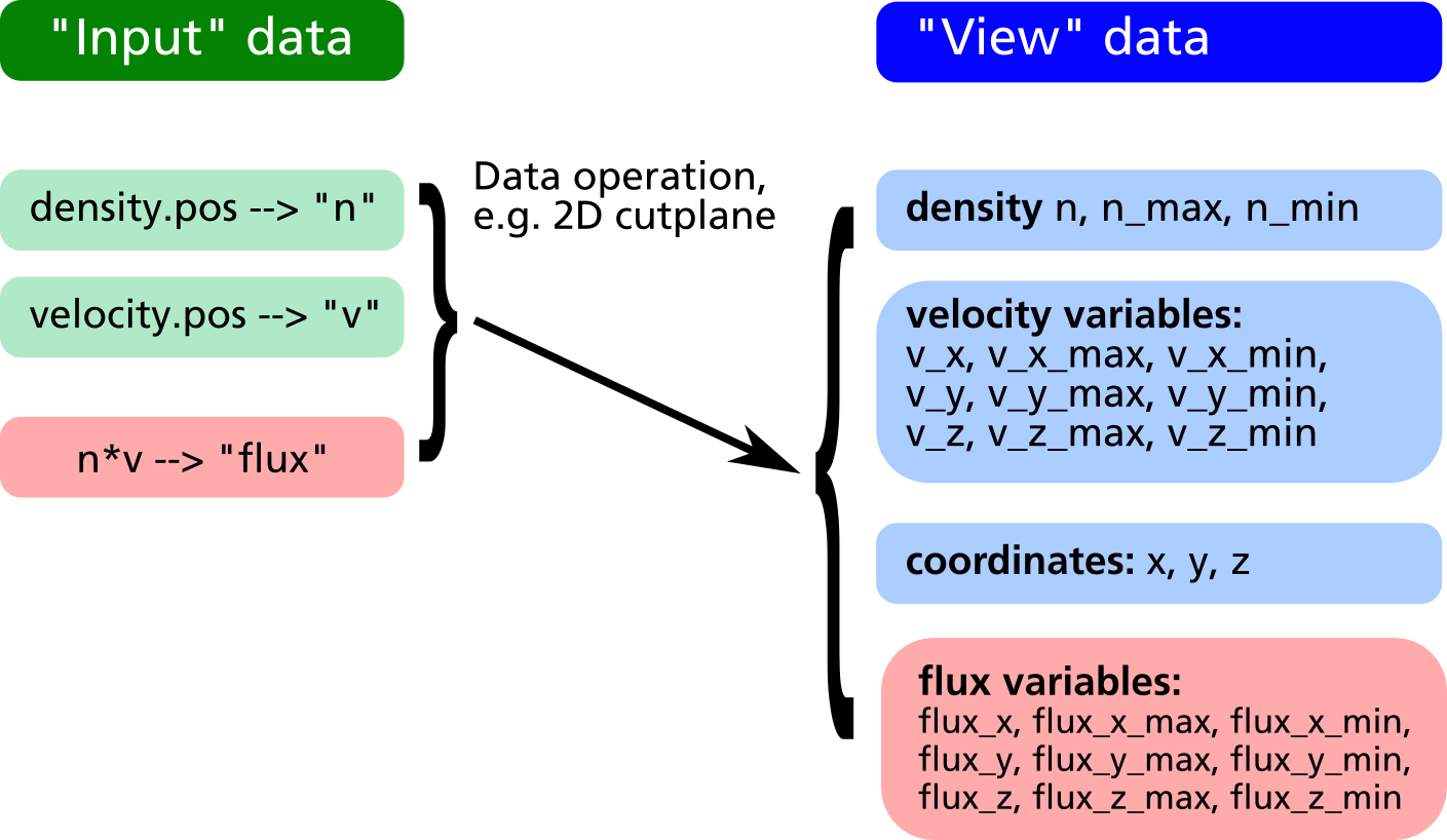
4.2.4.2 Reduction of input data
Let us assume we have 3D data of the density and velocity of evaporated atoms. In the XY-plane at Z=100 there is a substrate where the evaporated atoms can condensate.
First, in order to get the thickness profile on the substrate, the flux has to be extracted by multiplying density and z component of velocity in a cut-plane just below the substrate surface.
Second, let us assume the substrate is moving into Y direction, i.e. we have a dynamic deposition. In such cases, only the linescan of the profile in X direction averaged over Y is of relevance.
In order to do this, in prior versions of the post processing module it was required to make the 2D cut plane first, save it into a temporary POS file, load this POS file into a second post processing object and finally extract the line profile from there.
From version 2.4.3 on, there is the possibility of reducing the input data according to the last executed geometric operation, the command syntax is:
obj.reduce();
Reduction of input data space according to current arrangement of view data.
This allows for obtaining a line profile from 3D data in a much easier way:
compiletime load "module_ppp.so";
PPP obj = {};

aperture_width = 100;   # Aperture width on substrate in transport direction

obj.read("density.pos", "n");
obj.read("velocity.pos", "v");

# Define vertical flux component
obj.create_scalar("Fz", n*v_z);

# Make cut plane of data just below the substrate surface
obj.xy_plane(99.5, 10, "nearest_neighbour");

# Reduce input data to cut-plane (this is the important command)
obj.reduce();

# Make another cut plane averaging over the aperture_width
# in order to get the line profile
obj.xz_plane(0, aperture_width/2, "average");

# Write line profile into TXT file
obj.write_txt("absorption_line.txt",
              ["x", "avg_absorption", "rel_absorption"],
              [x, Fz, 100*Fz/Fz_max]);
4.2.4.3 Control of written data
Regarding the format of written data, there are the following possibilities:
- The coordinates, where the written data get plotted in POS files, can be explicitely specified
- It is possible to set a flag deciding whether to write data at a given coordinate point or not
The first option involves the following output methods:
obj.write_pos_scalar_parametric("filename.pos", "Legend", x, y, z, expression);obj.write_pos_scalar_binary_parametric("filename.pos", "Legend", x, y, z, expression);obj.write_pos_vector_parametric("filename.pos", "Legend", x, y, z, exp_x, exp_y, exp_z);obj.write_pos_vector_binary_parametric("filename.pos", "Legend", x, y, z, exp_x, exp_y, exp_z);
The first two commands are for parametrized scalar plots (in ASCII and binary format, respectively), the second two commands are for vector plots. An example is given in the following listing.
compiletime load "module_ppp.so";

PPP obj = {};
obj.read("density.pos",  "n");
obj.read("velocity.pos", "v");
obj.xy_plane(100, 10, "nearest_neighbour");

# Plot density and flux side by side. A coordinate offset allows for
# loading both pos files into GMSH and have the cut planes non-overlapping

obj.write_pos_scalar_binary_parametric("density-2D.pos", "Density [1/m^3]",
                                       x, y, z, n);
obj.write_pos_scalar_binary_parametric("flux-2D.pos", "Flux [1/m^3]",
                                       x+200, y, z, n*v_z);
In order to control explicitely, which data point should be written and which should be omitted, there is the possibility to define a write_flag variable within the postprocessing object. This is demonstrated in the following:
compiletime load "module_ppp.so";

PPP obj = {
  write_flag: A>0;
};

obj.read("absorption.pos", "A");
obj.write_pos_scalar_binary("absorption-noZeros.pos", "Absorption [1/m^2 s]", A);
In a large 3D absorption file, non-zero values only occur at the intersection between volume grid and mesh elements of walls. Thus a large fraction of the POS file consists of zeros, which is a waste in memory consumption. With the above script, the write_flag variable forces the write routine to only output those values with non-zero absorption, i.e. A>0.
It is important to define write_flag with a colon and not to write write_flag = (A>0);. In the rvm scripting language, the colon means that the value of write_flag will be only computed on request according to the currently defined parameters on right side. With the regular "=" assignment operator, the value of the variable A will be required at the moment of the definition of write_flag, which is not the case in the above script.
It is also possible to combine multiple conditions e.g. in order to specify a certain coordinate range for output:
compiletime load "module_ppp.so";

PPP obj = {
  write_flag: (abs(x)<100) and (y>-50) and (y<150);
};

# ...
4.2.4.4 Convolution function
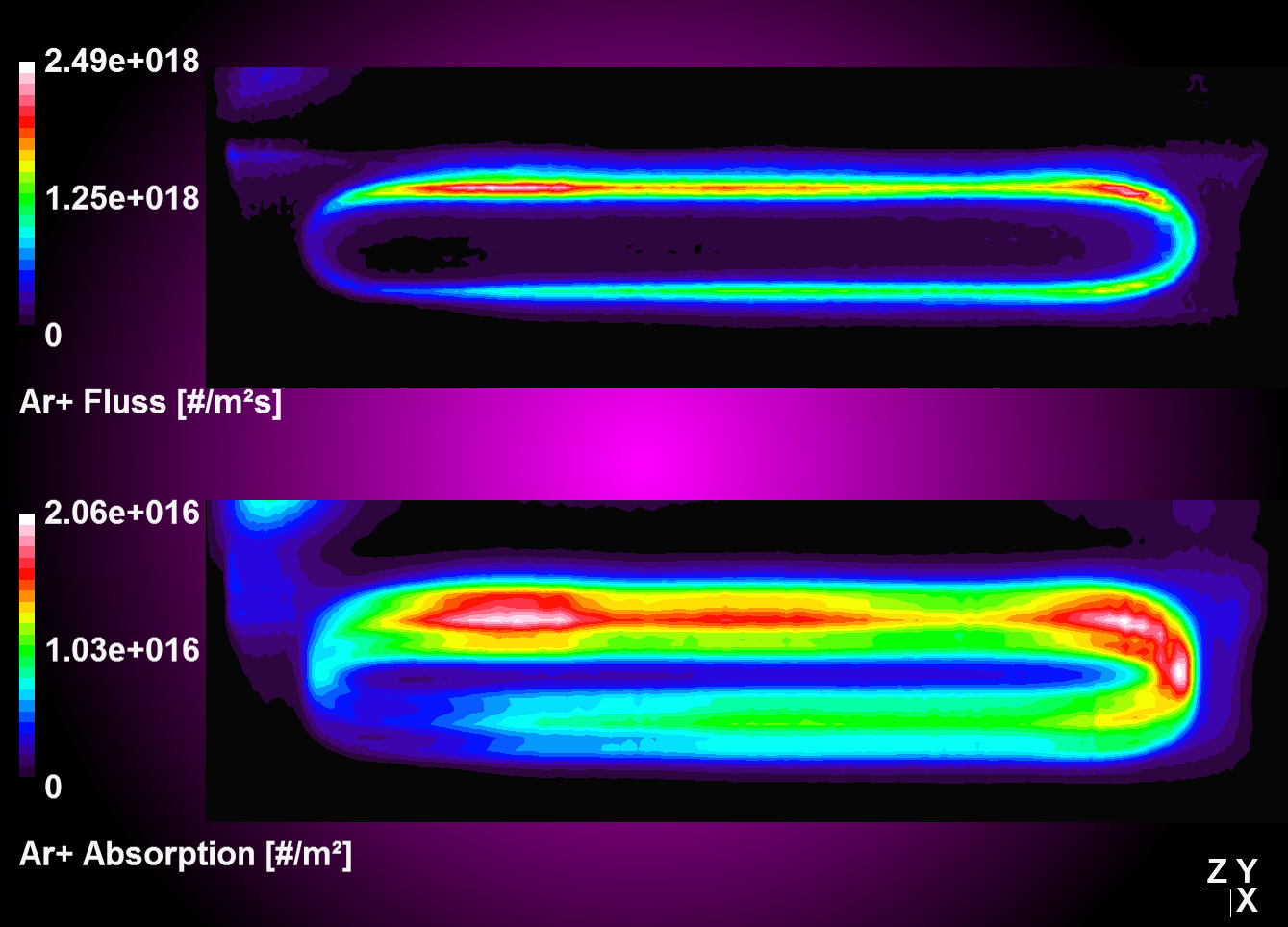
A convolution function has been implemented to operate on target absorptions plots in an attempt to model erosion profiles in MoveMag aplications. The primary approach here is to assume plasma and ion bombardment, respectively do not change with magnetron position which should be valid for small displacements vectors. Thus, we simply integrate over time the convolution of a time deviant, i.e. moving absorption plot with a stationary step function.
| Convolution and integration over time of moving source data with stationaly step function | Absorption plot (top) and convolution result (bottom) for a periodic oscillation in y |
|---|---|
 |
 |
compiletime load "module_ppp.so";

PPP obj1 = {};

#Define velocity vector and integration time
float vx[4], vy[4], vz[4]; #[m/s]
float T = 4; #[s]

#Oscillation starting from center position
#Move 1s to left with 1 m/s, then 2 times to right accordantly, then left again.
vx[0] = -1;
vx[1] = +1;
vx[2] = +1;
vx[3] = -1;

obj1.read("absorption_Arplus_100.00us.pos", "val");

obj1.xz_plane(0.0088, 1, "nearest_neighbour");

obj1.reduce; #Operate on cut plane (2D) data set for better performance!

obj1.convolution(vx, vy, vz, T, 0);

obj1.write_pos_scalar_binary("absorption_Arplus_100.00us_convolution.pos", val);
4.2.4.5 Convolution with linear weighting
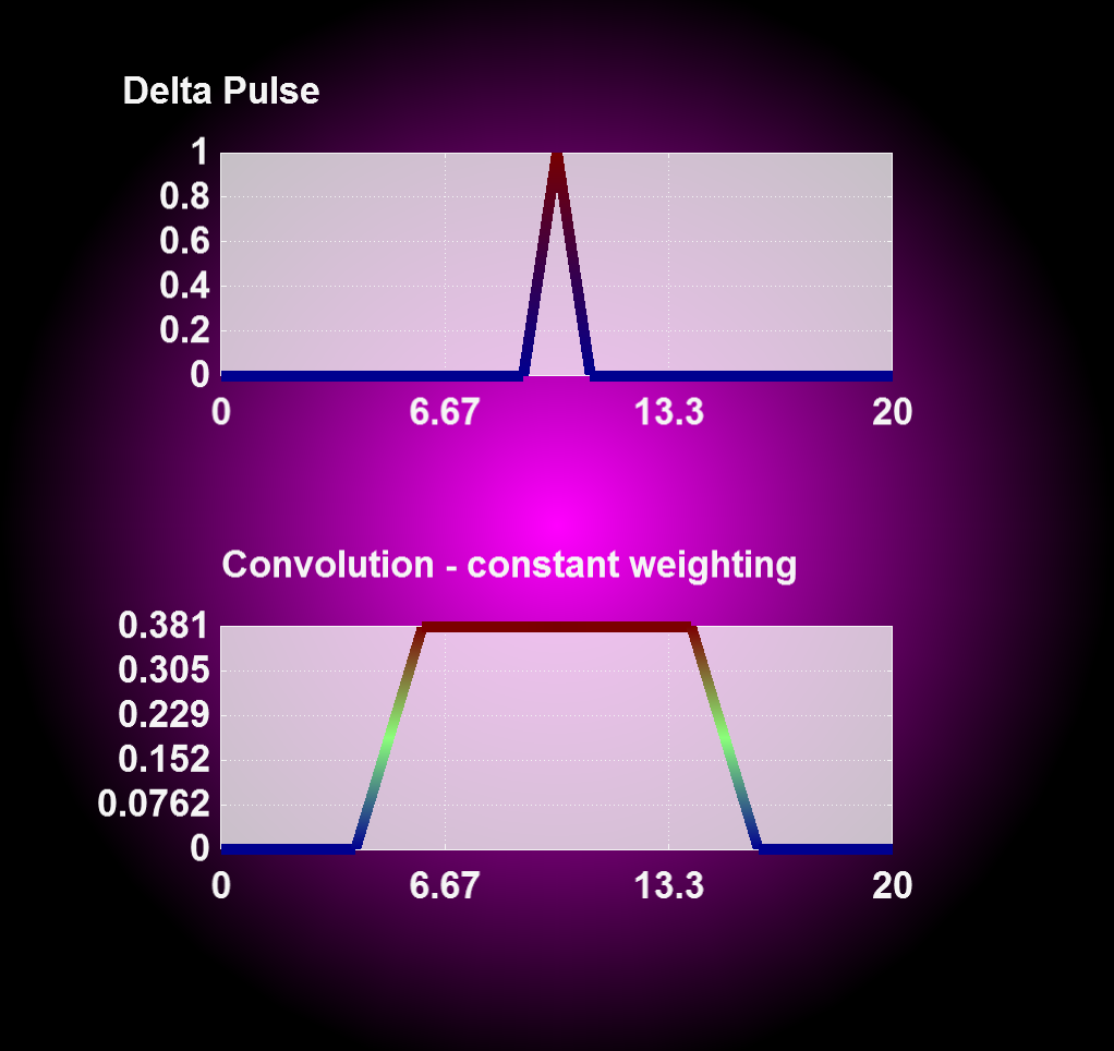
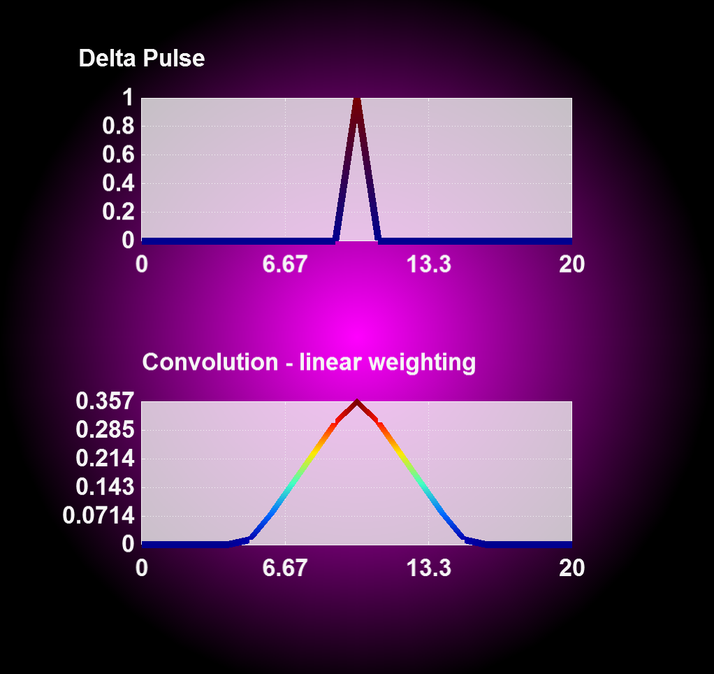
Entering '1' for the weighting flag enables a linear weighting scheme during convolution operation from 1 (no displacement) to 0 (maximum displacment). With this you can realize an interpolation between two or more states, i.e. magnetron positions, by merging the results from corresponding convolution operations together.
| Convolution with constant weighting | Convolution with linear weighting |
|---|---|
 |
 |
4.2.4.6 Circular Convolution
For a 360° convolution over the plot center use the function 'convolution_circular()' as seen below. This function has been implemented to adress modeling of absorption profiles on rotating substrates.
compiletime load "module_ppp.so";

PPP obj1 = {};

obj1.read("absorption_Arplus_100.00us.pos", "val");

obj1.xz_plane(0.0088, 1, "nearest_neighbour");

obj1.reduce; #Operate on cut plane (2D) data set for better performance!

obj1.convolution_circular();

obj1.write_pos_scalar_binary("absorption_Arplus_100.00us_convolution.pos", val);| Source data | After circular convolution |
|---|---|
 |
 |
obj.create_scalar("variable_name", expression);
obj.create_vector("variable_name", expression_x, expression_y, expression_z);

result = obj.integrate(expression);
obj.identity();
obj.reduce();
obj.convolution(vx, vy, vz, T, interpolation);
obj.convolution_circular();
4.3 Parametrized postprocessing with RIG-VM by examples
4.3.1 Simple scalar cut-plane
One of the easiest and most frequent tasks is to create a quick cut-plane aligned parallel to XY, XZ or YZ plane. Assumed, we have the file pressure_Ar_60.00ms.pos from a DSMC run of the tube example as output file, and would like to have a scalar pressure plot in the XY plane. The according script - let's call it extract.r looks like follows:
compiletime load "module_ppp.so";
case = BATCH.file;
time = 60;
PPP obj = {};

obj.read("$case/pressure/pressure_Ar_$(time%,2f)ms.pos", "pAr");
obj.xy_plane(0, 10, "nearest_neighbour");
obj.write_pos_scalar_binary("extract/$case-pressure_xy.pos",
                            "Ar pressure [Pa]", pAr);
In order to run this script with rvm, a subfolder extract should be in place. An example session is shown in the following, it assumes that the simulation parameter file is named tube.par and the post processing script is cutplane.r.
ap@sim159:~/sim/examples/ex1-tubeflow$ rvm -b cutplane.r tube
Created View {pAr}
File tube/pressure/pressure_Ar_60.00ms.pos has 96000 scalar and 0 vector points
XY-Plane extract, z0 = 0 +/- 10, method = 'nearest_neighbour'
Writing 'Ar pressure [Pa]' into scalar file 'extract/tube-pressure_xy.pos'
(2400 of 2400 points)
As result, the output file extract/tube-pressure_xy.pos is created and can be viewed in GMSH.
The meaning of the commands in the last three lines is as follows:
obj.read("input.pos", "variable_name");- The first parameter is the filename of the binary POS file
- The expression
$(time%,2f)will be replaced by the value of the variabletimewith 2 digits, i.e.60.00. - The second parameter is a variable name used for referencing these data in a later step
obj.xy_plane(0, 10, "nearest_neighbour");- Create a cutplane parallel to the XY coordinates and positioned around z=0 (first parameter)
- Consider each point in a search radius \(z = 0 \pm 10\) on both sides of the cutplane and
- Display the nearest point onto the cutplane
obj.write_pos_scalar_binary("output.pos", "plot_title", expression);- This writes a scalar output file named
"output.pos". - The
"plot_title"will be shown as view title in GMSH. - With
expressionthe scalar output value can be specified. In the above example, it is just the pressure value namedpAr.
- This writes a scalar output file named
Besides of obj.xy_plane(z0, delta_z, "method") there are also obj.xz_plane(y0, delta_y, "method"); and obj.yz_plane(x0, delta_x, "method"); available.
4.3.2 Scalar cut-plane with arithmetics
Within the expression parameter it is possible to do some arithmetics. If e.g. the pressure should be plotted in mTorr instead of Pa (1 mTorr = 133 mPa), the following script will do it:
compiletime load "module_ppp.so";
case = BATCH.file;
time = 60;
PPP obj = {};

obj.read("$case/pressure/pressure_Ar_$(time%,2f)ms.pos", "pAr");
obj.xy_plane(0, 10, "nearest_neighbour");
obj.write_pos_scalar_binary("extract/$case-pressure_xy.pos",
                            "Ar pressure [mTorr]", pAr*1000/133);
4.3.3 Scalar cut-plane with triangulation
By replacing the command write_pos_scalar_binary by write_pos_triangulate it is possible to create a triangulated scalar view:
compiletime load "module_ppp.so";
case = BATCH.file;
time = 60;
PPP obj = {};

obj.read("$case/pressure/pressure_Ar_$(time%,2f)ms.pos", "pAr");
obj.xy_plane(0, 10, "nearest_neighbour");
obj.write_pos_triangulate("extract/$case-pressure_xy.pos",
                            "Ar pressure [mTorr]", pAr*1000/133);
4.3.4 Scalar cut-plane from multiple input files
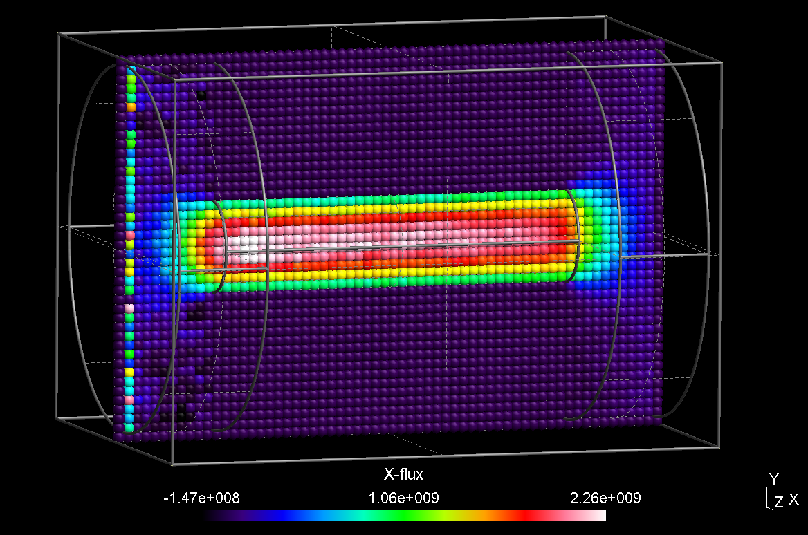
Let’s assume we would like to plot the flux (=density*velocity) in positive X direction and have the density as well as the number plots activated. Arithmetics in the postprocessing script allow to compute the density from the particle number and from that the flux:
compiletime load "module_ppp.so";
case = BATCH.file;
time = 60;
PPP obj = {};

obj.read("$case/number/number_Ar_$(time%,2f)ms.pos", "N");
obj.read("$case/velocity/velocity_Ar_$(time%,2f)ms.pos", "v");
obj.read("$case/cell_volumes.pos", "vol");
obj.xy_plane(0, 10, "nearest_neighbour");
obj.write_pos_triangulate("extract/$case-xflux_xy.pos",
                          "Ar flux [1/m^2s]",
                          vol>0 ? 8e12*N/vol*v_x ! 0);
The velocity is a vector plot; thus, by reading in the velocity with variable name v, the three vector components v_x, v_y, v_z are internally created and can be used in the expression arithmetics. The density is computed from the number N as 8e12*N/vol, where 8e12 is the scaling factor NREAL_Ar between real and simulated number of Ar atoms. However, for some simulation cells, which are fully contained within a wall of the geometric model, the volume vol is zero and thus, the above expression will fail. Therefore, the expression for the density contains an implitic if statement in the form vol>0 ? ... ! .... The expression after the ? is taken, if vol>0 holds, otherwise the expression after the ! is computed instead.
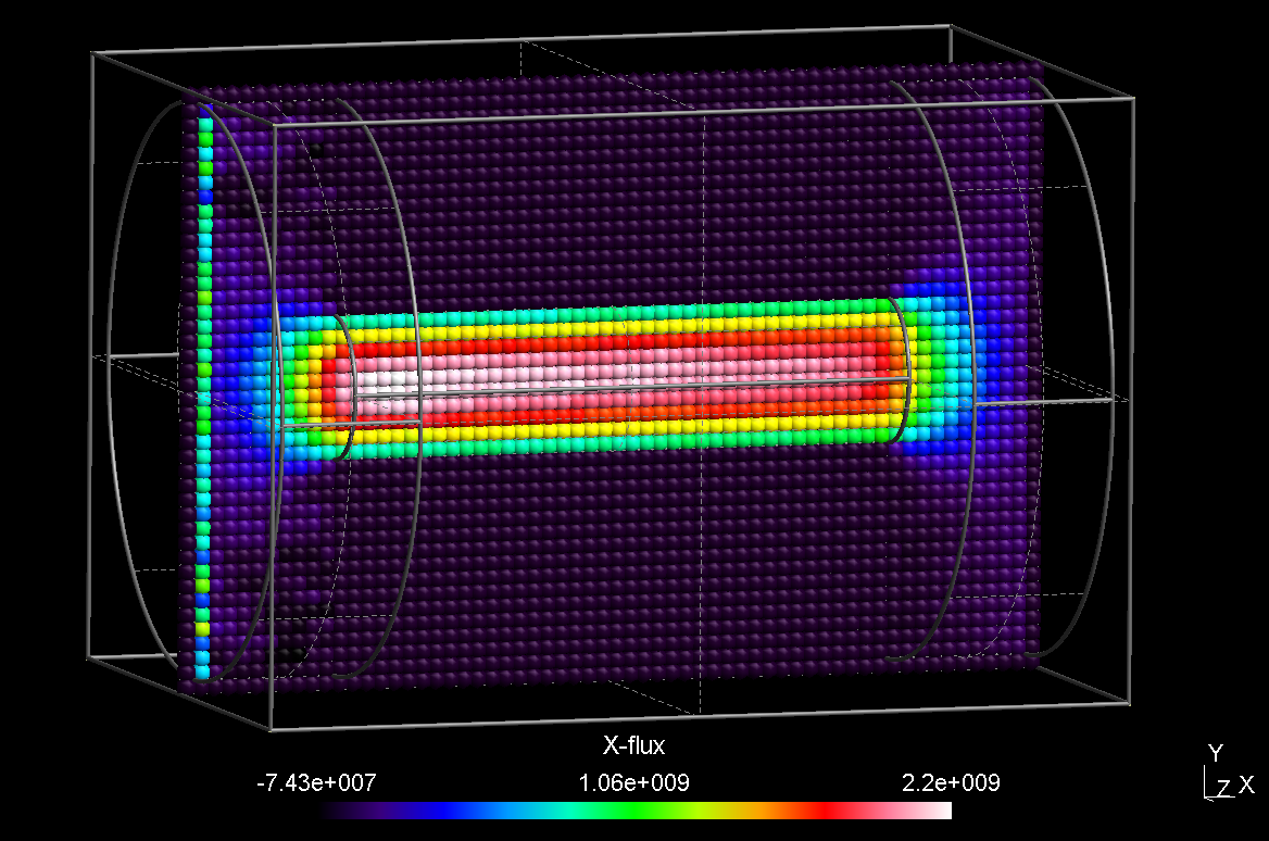
Depending on the statistics, the cut-plane of the flux plot may look a bit noisy. In this case, it helps to use the "interpolate" option rather than "nearest_neighbour":
obj.xy_plane(0, 10, "nearest_neighbour"); |
obj.xy_plane(0, 10, "interpolate"); |
|---|---|
 |
 |
Putting all the arithmetics into the expression argument can get confusing. There are multiple ways to define the density expression separately, one method is to define it within the PPP object:
compiletime load "module_ppp.so";
case = BATCH.file;
time = 60;
PPP obj = {
  float NREAL = 8e12;
  float nAr: vol>0 ? NREAL*N/vol ! 0;
};

obj.read("$case/number/number_Ar_$(time%,2f)ms.pos", "N");
obj.read("$case/velocity/velocity_Ar_$(time%,2f)ms.pos", "v");
obj.read("$case/cell_volumes.pos", "vol");
obj.xy_plane(0, 10, "nearest_neighbour");
obj.write_pos_triangulate("extract/$case-xflux_xy.pos",
                          "Ar flux [1/m^2s]", nAr*v_x);
Since the variables N and vol are not known during definition of nAr within the PPP object, it is important to use the alias method (i. e. the ":") instead of the assign method (i. e. "=") for definining density. The result of this modified script is the same as for the script above but now, it looks more clearly arranged.
Another way is to create an input data set of the density via the create_scalar method:
compiletime load "module_ppp.so";
case = BATCH.file;
time = 60;
PPP obj = { };

obj.read("$case/number/number_Ar_$(time%,2f)ms.pos", "N");
obj.read("$case/velocity/velocity_Ar_$(time%,2f)ms.pos", "v");
obj.read("$case/cell_volumes.pos", "vol");

obj.create_scalar("nAr", vol>0 ? 8e12*N/vol ! 0);

obj.xy_plane(0, 10, "nearest_neighbour");
obj.write_pos_triangulate("extract/$case-xflux_xy.pos",
                          "Ar flux [1/m^2s]", nAr*v_x);
4.3.5 Time averaging
In order to perform averaging of the same quantity over several time steps, it is sufficient to call the function obj.read(...) several times but with the same variable name. An example is given in the following:
compiletime load "module_ppp.so";
case = BATCH.file;
T1 = 100; T2 = 200; DT = 10;
time = 60;
PPP obj = {
  float NREAL = 8e12;
  float nAr: vol>0 ? NREAL*N/vol ! 0;
};

for (time=T1; time<=T2; time=time+DT) {
  obj.read("$case/density_Ar_$(time%,2f)ms.pos", "d");
  obj.read("$case/velocity_Ar_$(time%,2f)ms.pos", "v");
}
obj.read("$case/cell_volumes.pos", "vol");
obj.xy_plane(0, 10, "nearest_neighbour");
obj.write_pos_triangulate("extract/$case-xflux_xy.pos",
                          "Ar flux [1/m^2s]", nAr*v_x);
The read command of the PPP object automatically recognizes if one variable is used several times and performs an averaging of the data in this case.
4.3.6 Development over time
If you would like to illustrate the development of the same quantity over several time steps, you need to call obj.append(...) several times but with the same variable name and then one of the write_pos_time_steps functions. An example is given in the following:
compiletime load "module_ppp.so";
compiletime load "module_system_linux.so";

# defining parameters
case   = BATCH.file;
start  = 100;
end    = 200;
dtime  = 20;
unit   = "us";
z      = 0;
folder = "density";
files  = "density_e";

# create ppp subfolder if it does not exist
System FS = { rootpath = "$case"; };
if (FS.folder_exists("ppp") == 0) then {
  out "Creating folder $case/ppp\n";
  FS.create_folder("ppp", 493)
};

# applying a cut plane to each time step
for (time=$start; time<=$end+0.001; time=time+dtime) {
  PPP obj1 = {};

  obj1.read("$case/$folder/$(files)_$(time% 4,2f)$(unit).pos", "X");
  obj1.xy_plane($z, 10, "nearest_neighbour");
  obj1.write_pos_scalar_binary("$case/ppp/cut_$(files)_$(time% 4,2f)$(unit).pos",
                               "$files", X);
}

# appending the cut planes to each other
PPP obj2 = {};
for (time=$start; time<=$end+0.001; time=time+dtime) {
  obj2.append("$case/ppp/cut_$(files)_$(time% 4,2f)$(unit).pos", "Y");
}
obj2.write_pos_time_steps_scalar_binary(
  "$case/timestep_cut_$(z)mm_$(files)_$(start)-$(end)$(unit).pos", "$files", "Y"
);
First of all module_system_linux.so is loaded, which is needed for creating the ppp subfolder for storing the intermediate cut planes. Next some parameters are set including the time interval, the z position of the cut plane and the name of the plot. Then the ppp subfolder is created, where the cut planes generated in the next part are stored. In the last part these cut planes are appeded to each other and written to the output file.
The order of first creating the cut planes and then appending them to each other is important, because it is (at the moment) not possible to make cut planes of variables with multiple time steps. Additionally the write_pos_time_steps functions can only be called on the variable name and not on an expression, so that calculations have to be done before.
4.3.7 Generating vector plots as cut plane
Finally we would like to plot the flux as vector plot. All we have to do is to replace the obj.write_pos_scalar(...) by obj.write_pos_vector(...). Since a vector plot has three components, we have three instead of one expression arguments.
compiletime load "module_ppp.so";
case = BATCH.file;
time = 60;

PPP obj = {
  float NREAL=8e12;
  float density: vol>0 ? NREAL*N/vol ! 0;
};

obj.read("$case/number/number_Ar_$(time%,2f)ms.pos", "N");
obj.read("$case/velocity/velocity_Ar_$(time%,2f)ms.pos", "v");
obj.read("$case/cell_volumes.pos", "vol");
obj.xy_plane(0, 20, "interpolate");
obj.write_pos_vector("extract/$(case)-cutplane_xy.pos", "Flux (1/m^2 s)",
                     density*v_x, density*v_y, density*v_z);
4.3.8 Revert POS file data to original state
The obj.identity() function enforces to transfer the whole input data into the view data. It is only necessary to invoke this function, if the view data are reduced due to a previous data operation such as a cutplane. Without data operation, obj.identity() is internally invoked, automatically.
compiletime load "module_ppp.so";
case = BATCH.file;
time = 60;

PPP obj = {};

obj.read("$case/number/number_Ar_$(time%,2f)ms.pos", "N");
obj.xy_plane(0, 10, "nearest_neighbour");
obj.write_pos_scalar("cutplane_xy.pos", "Ar number [#]", N);
obj.identity();
obj.read("cell_volumes.pos", "vol");
obj.write_pos_scalar("density_Ar.pos", "Ar density [#/m^3]", vol>0 ? N/vol ! 0);
4.3.9 General (oblique) interpolation views
For cutplanes which are not parallel to one of the coordinate planes, it is possible to specify them in a more general way. For this purpose, a general description of a parametric plane looks as follows:
\[\vec{r}(s,t) = \vec{x}_0 + s\left(\vec{x}_1-\vec{x}_0\right) + t\left(\vec{x}_2-\vec{x}_0\right)\]{#eq:ppp_plane}
The accordant post processing command is written as:
obj.plane(x0, y0, z0, x1, y1, z1, x2, y2, z2, delta, N, M, "method");First, the three points of the above equation are given coordinate-wise (i.e. the first 9 parameters). The next parameter delta is the vertical distance to the plane, wherin points are considered for interpolation. The integer numbers N, M give the resolution of the cut plane in direction of the first and second vector. Update: It is possible to specify 0, 0 for N, M; in this case the actual resolution of the imported POS file will be taken.
An example of an oblique plane with respect to our tube DSMC case is shown in the following:
compiletime load "module_ppp.so";
case = BATCH.file;
time = 60;

PPP obj={
  float density: vol>0 ? N/vol ! 0;
};

obj.read("$case/number/number_Ar_$(time%,2f)ms.pos", "N");
obj.read("cell_volumes.pos", "vol");

obj.plane(-110, -210, -210,  200, 210, 0,  200, -210, 0,
          15,  40, 40, "interpolate");

obj.write_pos_scalar_binary("extract/$case-obliqueplane.pos",
                            "Density [1/m^2 s]", density);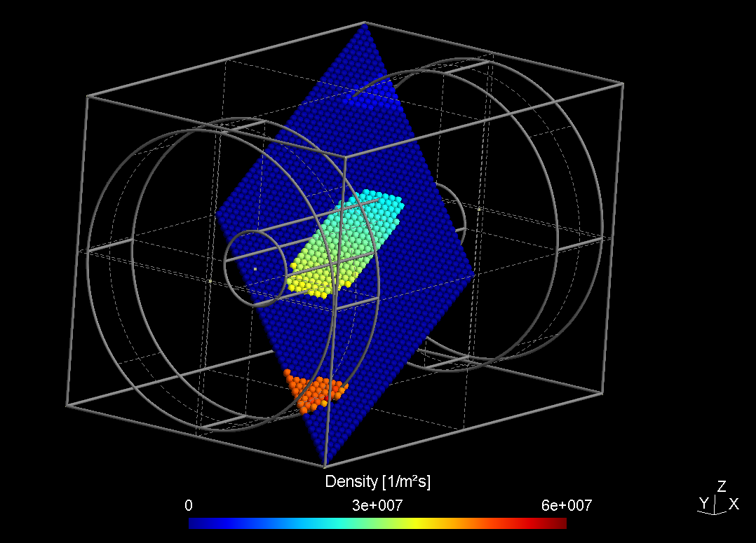
Analogously, it is possible to extract data along a straight line:
\[\vec{r}(s) = \vec{x}_0 + s\left(\vec{x}_1-\vec{x}_0\right)\]{#eq:ppp_line}
with the postprocessing command:
obj.line(x0, y0, z0, x1, y1, z1, delta, N, "method");4.3.10 Additional output formats
4.3.10.1 Visualization Toolkit (VTK)
Besides the POS output format of GMSH, it is possible to write the 3D data in the Visualization Toolkit format. The two functions for scalar and vector data are:
obj.write_vtk_scalar("output.vtp", "View title", expression);
obj.write_vtk_vector("output.vtp", "View title", expression_x, expression_y, expression_z);
The syntax is identical to that of the POS format.
4.3.10.2 Tecplot
Also the Tecplot format is supported for both scalar and vector data:
obj.write_tec_scalar("output.dat", "View title", expression);
obj.write_tec_vector("output.dat", "View title", expression_x, expression_y, expression_z);
Again the syntax is identical to that of the POS format.
4.3.10.3 ASCII *.TXT output
It is convenient to directly export certain results as ASCII TXT file, which can be imported e.g. in Origin or other graph presentation software. For that purpose, the following method is implemented:
obj.write_txt("file_name.txt", ["col1", "col2", ...], [exp1, exp2, ...]);The arguments have the following meaning:
- The first argument is the name of the TXT file, which should be created
- The second argument is a list containing all column title strings. They will appear in the first line of the ASCII file.
- The third argument is a list of expressions, which should be computed for each column.
- Within the expressions, all variable names originating from imported POS files as well as the variables "x, y, z" for the respective coordinates can be used.
- Additionally, the maximum and minimum values of all variables are computed and can be accessed via
variablename_max,variablename_min.
We demonstrate this in a short example:
compiletime load "module_ppp.so";

PPP obj1 = {};

obj1.read("absorption.pos", "A");
obj1.xy_plane(-141.75, 10, "nearest_neighbour");
obj1.write_pos_scalar_binary("absorption-2D.pos", "SiH4 absorption [1/m^2 s]", A);

PPP obj2 = {};

obj2.read("absorption-2D.pos", "A");
obj2.line(420, -380, -141.75,   607.5, -380, -141.75,  40, 19, "average");
obj2.write_txt("profile_avg.txt",
               ["r [mm]", "abs [1/m^2 s]", "abs [%]"],
               [x-420, A, 100*A/A_max]);
This script reads a 3D posfile "absorption.pos" of an absorption plot into obj1, creates a 2D cutplane of it and stores the cutplane into "absorption-2D.pos". This created file is then read into a second PPP object obj2. Here, the absorption profile is averaged along a line in X direction. The averaged profile is finally dumped into an ASCII file. The ASCII file finally looks like follows:
         r [mm]   abs [1/m^2s]        abs [%]

        4.93421    3.80416e+20        99.9454
        14.8026    3.77636e+20        99.2152
        24.6711    3.80623e+20            100
        34.5395     3.7374e+20        98.1916
        44.4079    3.75455e+20         98.642
        54.2763    3.73143e+20        98.0347
        64.1447    3.68571e+20        96.8336
        74.0132    3.63662e+20        95.5439
        83.8816    3.58961e+20        94.3087
          93.75    3.54935e+20         93.251
        103.618    3.47403e+20         91.272
        113.487    3.43792e+20        90.3235
        123.355    3.31429e+20        87.0752
        133.224    3.24909e+20        85.3624
        143.092    3.18416e+20        83.6563
        152.961    3.03792e+20        79.8144
        162.829    2.88857e+20        75.8905
        172.697    2.66338e+20        69.9741
        182.566    2.29174e+20        60.2102
4.3.10.4 CSV output
Instead of TXT files, writing the output in the CSV format is also possible. The syntax of write_csv is identical to that of write_txt:
obj.write_csv("file_name.csv", ["col1", "col2", ...], [exp1, exp2, ...]);The column separator is a colon, which is explicitely mentioned in the file and the decimal separator is a point.
4.3.11 Numerical integration
The numerical integration feature is currently available for cut-planes only. In our tube example we might want to integrate the particle flux through the tube. This can be accomplished as follows:
compiletime load "module_ppp.so";

mesh_unit=1e-3;
Nsccm = 4.478e17;

file "integration.txt" << for (time=20; time<=400; time=time+20) {
  PPP obj={};
  obj.read("density_Ar_$(time).00ms.pos", "density");
  obj.read("velocity_Ar_$(time).00ms.pos", "v");
  obj.plane(200, -60, -60,   200, 60, -60,   200, -60, 60,
            10, 0, 0, "interpolate");
  flow = obj.integrate(density*v_x)*mesh_unit^2/Nsccm;
  out "$(time)  $(flow)\n";
}
In the script shown above, the density and velocity of Argon are loaded for a complete time series t=20...400 ms. For each time step, a PPP object is created, and the flux is generated via the expression density*v_x within the cut plane. With the integrate function, the total flux through the tube cross section can be computed.
The numerical integration is internally performed over triangles of adjacent points. For each triangle, the average of the three point values is multiplied with the area of the triangle element. If the mesh unit is not 1 m, the integration result should be multiplied with mesh_unit^2 in order to get the correct unit.
In the example script, the result is additionally divided by the particle number per second for 1 sccm in order to get the flow in sccm.
4.3.12 Merging of (position) plots
In the normal output files (e.g. density) each point corresponds to a single cell with its position and its value. A second density plot has the same cells at the same position but with different values. Therefore it makes no sense to merge these files into a single one, this is only the case for position plots, where the positions of particles are stored independent of the cell resolution. By merging multiple of these files the illustration of the particle movement is possible:
compiletime load "module_ppp.so";

PPP obj = {};

for (float time=0; time<=100; time=time+0.5) {
  obj.merge("position/position_e_$(time %,2f)ns.pos", "pos");
 }
obj.write_pos_scalar_binary("position_e_0-100ns.pos", "e position", pos);
In this example a position plot each 0.5 ns for a time interval between 0 and 100 ns is merged and written to a single file. The syntax of the merge function is identical to that of the read function.
4.4 Parametrized postprocessing with GMSH
4.4.1 Creating animated image sequences in GMSH
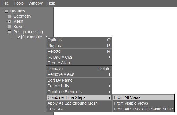
As first step, multiple successive views have to be loaded into gmsh and combined into a sequence with the command Combine Timesteps->From All Views (see Fig. 3). The command From Visible Views would only consider the views with an active checkbox in front. Another possibility to combine plots would be to use one of the write_pos_time_steps() functions from the RVM postprocessing module.
The next step is to create a GMSH script which subsequently saves each image of the sequence as PNG file. A possible example of such a script is given in the following:
Print.Background       =  1; // Use this, if the background color should be included
General.GraphicsWidth  =  1280;
General.GraphicsHeight =  720;

Steps = View[0].NbTimeStep; // Automatic determination of the number of time steps

For Num In {0:Steps-1}
  View[0].TimeStep = Num;
  Draw;
  Print Sprintf("ani-%02g.png", Num);
EndFor
With Windows Movie Maker these PNG files can be combined into a WMV film sequence. Another possibility is the use of Blender which is described in next section. For creating animated GIFs, the linux tool convert from the ImageMagick package can be used as follows:
convert -delay 20 -loop 0 ani*.png output.gifWith the -delay switch, the time delay between frames can be specified in 1/100 seconds. The switch -loop 0 creates an endless loop.
4.4.2 Creating animations with Blender
With the free and open-source 3D computer graphics software program Blender it is easily possible to create short animations from images extracted from GMSH. Although the program is much more powerful it is also suitable for our purpose. In the following, a step-by-step tutorial is given.
4.4.2.1 Step 0
Download, install and open the software Blender.
4.4.2.2 Step 1
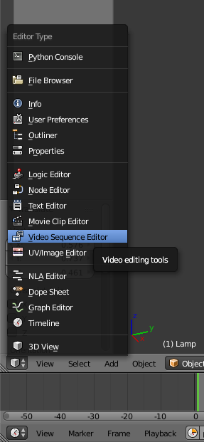
On the left bottom side click on the cube icon and open the Video Sequence Editor.
4.4.2.3 Step 2
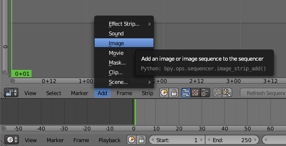
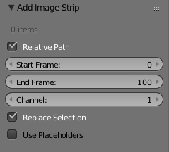
Click on Add and Image to choose the images extracted from GMSH.
4.4.2.4 Step 3
Navigate to the folder where the images are located and select them simply by making multiple selection boxes (hold left mouse button and drag). Now you have to edit the box in the lower left corner and adjust the start and end frame to your case.
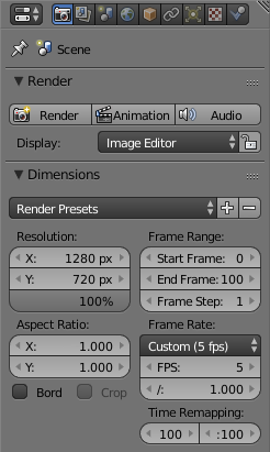
4.4.3 Step 4
Then you have to open the render menu on the right by clicking on the camera symbol. Now the dimensions of the animation have to be set. Depending on the resolution of your images edit the X and Y value and set the percentage to 100. In the frame range you should use the same values as in step 3. The frame rate namely the images shown per second you can adapt to your means, nevertheless a value of 5 is a good starting point.
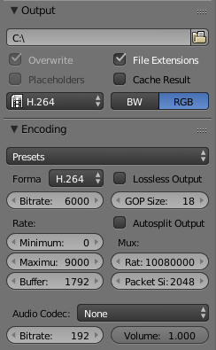
4.4.4 Step 5
Now the output path and the file format have to be set. For the file format H.264 is a good choice and you should select RGB for a coloured animation. In the encoding menu also select H.264 as the format.
4.4.5 Step 6
That's it, if you now click on Animation in the render menu your video is created.

The acronym PPP stands for PIC-MC Postprocessing.↩︎