DSMC and PICMC documentation
2024-09-20
6 Particle-in-Cell Monte-Carl (PIC-MC) examples
6.1 1D - HF parallel plate discharge benchmark case
A simple 1D setup in Argon with one grounded and one HF excitated parallel plate is provided in this ZIP file. This setup has been motivated by (Turner et al. (2013)) in order to compare results from our code against other reference implementations.
6.1.1 Starting the simulation
The setup file contains four parameter files P1.par, P2.par, P3.par and P4.par which can be started with up to 8 CPUs each. Start the simulation (e.g. P1.par) with:
$ rvmmpi -picmc 8 P1.par6.1.2 Results
The simulation yields, among other results, electron and Ar+ density profiles along the 1D axis, which can be compared against accordant benchmark results (Turner et al. (2013)) (see Table. (tbl:picmc_turner1d?), left graph).
For this example, we can see a certain impact of the choice of the energy partitioniong model (see special parameters) on the low-pressure case P1. While in our implementation the simpler one takes it all model is selected by default, it results in significat deviations to the implementation in Turner et al. (2013) under certain conditions. In contrast, with the equal share model, there’s practically no deviation visible (see Table (tbl:picmc_turner1d?), right graph).
The real physical behaviour might be a mixture between both models. We are currently not aware if that can be decided on the basis of known experimental data.
| Comparison against benchmark results | Impact of electron energy partitioning model |
|---|---|
 |
 |
6.2 BEM - magnetic field computation
The field problem of a permanent magnet arrangement, according to (Jackson (1999)) is the solution of the Poisson equation for a magnetostatic scalar potential to be formulated. The magnetization of the permanent magnets is assumed in good approximation as homogeneous and replaced by an equivalent magnetic surface charge. The distribution of surface charges and magnetic permeability in the computational domain is the source term of the Poisson equation. With an appropriate definition of boundary conditions, the magnetostatic field problem is fully described.
For the numerical calculation of the Poisson equation the boundary element method (BEM) is used. This method does not need to be discretized as finite differences or finite element method, the entire computational volume, but only the surface of the computational domain. The method of boundary elements is therefore particularly suitable for field problems with open boundary conditions in an infinite computational domain. Another advantage of this method is the high accuracy over the above-mentioned volume methods, but are paid for with increased memory and computational effort.
6.2.1 Usage
The boundary element method (BEM), how we implemented it, can be used also for electrostatic field problems without space charges. However it has been primarily developed for magnetostatic field problems, i.e. magnetic fields from permanent magnet arrangements. Thus, we exemplarily show the application of the BEM field solver for a simple rectangular magnetron setup in this section.
First we have to define the geometric model using GMSH. Hereby some modeling constraints have to be taken into account slightly different to that of the DSMC and PIC-MC simulation respectively. From the meshed surface model a parameter file is created automatically which has to be adjusted manually. Finally the computation can be executed via a console command. In the following subsections these subsequent steps are described in more details.
6.2.1.1 Geometry modelling
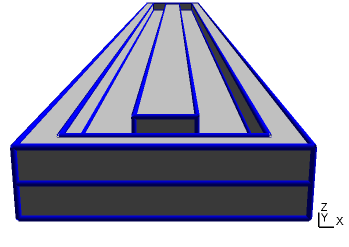
We exemplarily take an simple planar magnetron setup and create a geometry model using GMSH. The end section of the planar magnetron assembly is shown in Figure (fig:picmc_pk750_photo?).
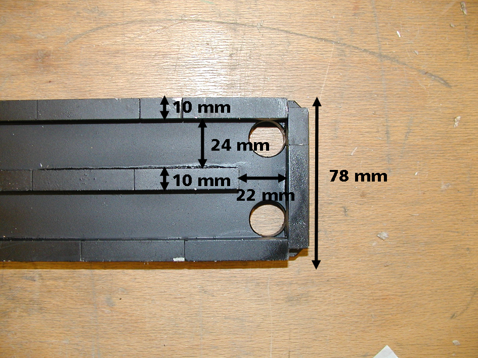
The first thing to do is to determine the number of domains, i.e. number of self-contained material areas. In the current case, we have (i) vacuum, (ii) magnets and (iii) yoke. Unless you have magnets with different permeabilities, all magnets can be attributed to the same domain. For each domain there is an interface to at least another adjacent domain. Additionally, for the magnets we need an interface for the top surface, the bottom surface and the skin surface. The top and bottom surfaces will later be specified as north and south pol; thus, they have to be separated from the skin surfaces.
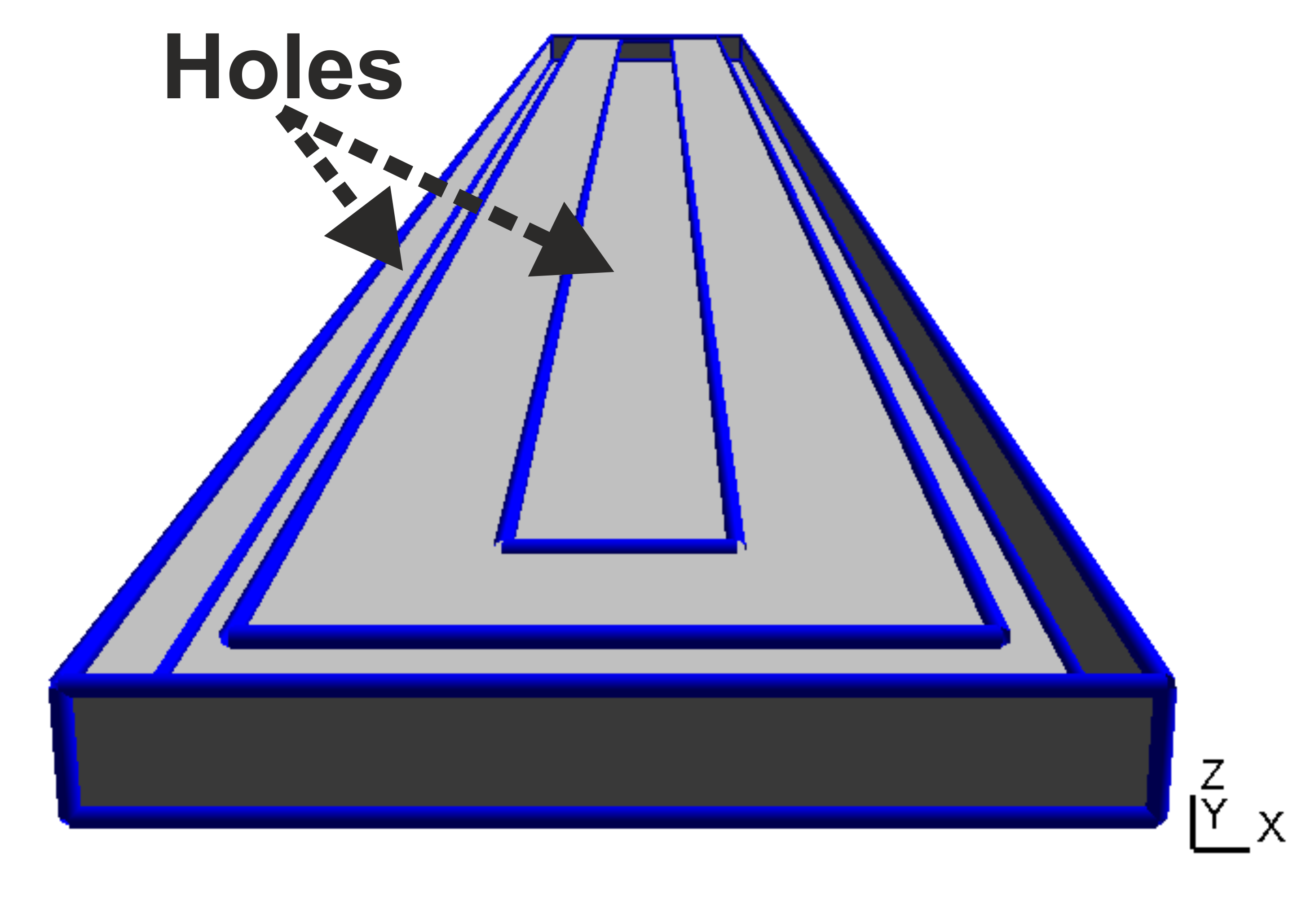
In our case we have six interfaces: (1) from the yoke to the vacuum, (2) from the magnet skin surfaces to the vacuum, (3) from the outer magnet top surface to the vacuum, (4) from the outer magnet bottom surface to the yoke, (5) from the inner magnet top surface to the vacuum and (6) from the inner magnet bottom surface to the yoke.
Step 1: Create or load a geometric surface model with GMSH.
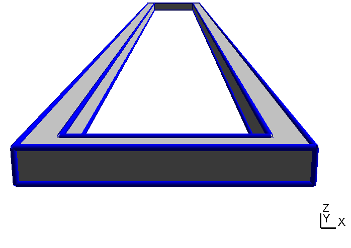
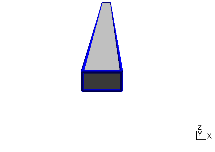
Now when we create the geometry model with GMSH we define one and only one geometrical surface for each interface. Thus, in our case the upper surface of the yoke has two "holes" for the bottom surfaces of the inner and the outer magnet as shown in Table (tbl:picmc_pk750_assembly?).
| Yoke | Outer magnet | Inner magnet | Complete magnet assembly |
|---|---|---|---|
 |
 |
 |
 |
When all geometric surface are defined they must be grouped accordantly and assigned to a string tag. Read the GMSH instructions on how to define physical surfaces from geometric surfaces. After the physical surface definition the geometric model can be meshed (2D mesh, press the “2” button) and saved. In short, there are the following general rules for setting up a magnetron geometry:
- Magnets should always be constructed as a closed body.
- If a magnet directly touches a yoke, there should be only one surface between the magnet and the yoke.
- Alternatively it is also possible to leave a tiny gap (gap with 1/10 mm or less) between magnet and yoke, this is often a good workaroud in case of complicated yoke geometries
6.2.1.2 Parameter file settings
If a magnetic field computation is performed, there are always two different meshfiles required:
- One meshfile for the magnetic arrangement itself, let’s call it magnet.msh
- Another meshfile, where the geometric region of interest is defined. This is the region, where the magnetic field vectors should be computed and where later on a plasma simulation will be performed. Let’s call the second meshfile chamber.msh.
Step 1: Create a parameter file. To generate a parameter file for the BEM field solver first execute the command on the mesh-model for plasma simulation:
initpicmc chamber.msh whereas chamber.msh is the accordant mesh file to define the computation domain for plasma simulation and electric field computation, respectively (i.e. the second meshfile mentioned above). This command generates a parameter file named chamber.par in the same directory. All definitions regarding computation domain, cell spacing, cell resolution, number of subquads, etc., are defined within this parameter file. The region of interest for magnetic field should be the same computation domain and cartesian grid, respectively as for plasma simulation. Thus, by deriving parameter file for magnetic field computation from primary parameter file, twofold definition is avoided. Hence, you have to find the section where mesh files are defined and insert a chamberfor the magnetic mesh-model you want to use. The section looks like this:
MESHFILE = "chamber.msh";   # Name of mesh file for PICMC particle simulation
BEMMESH  = "";              # Name of mesh file for BEM b-Field solver
Insert the proper filename, e.g. magnet.msh in the empty quotes next to the BEMMESH tag. Remember that mesh files must be in same directory as parameter files. Now execute the command:
initbfield chamber.parThis command creates a template for the magnetic fieldsolver named chamber.bem in the same directory.
Step 2.0: Edit magnetic definition file chamber.bem.
The parameters which have to be adjusted in chamber.bem are:
- The relative permeability of every domain, e.g. 1.05 for the magnets or 1000 for the yoke. These are the entries in the
Domainsarray. - The definitions for all surfaces defined in the magnetic mesh-model. This is the tricky part, because you have to connect interfaces surfaces manually by using the prober domain numbers. Also you have to define the magnetic remanence, if any, on the accordant surfaces. All surface definitions take place within the record entry
Codecs.
Step 2.1: Set number of domains and domains’ relative permeability, respectively.
The magnetron example from above section consists of three domains:
- The vacuum with a relative permeability of 1.0.
- The magnets with a relative permeability of 1.05 (found in the datasheet for the magnets).
- The yoke of ST37 steel with high relative permeability, i.e. we set it to 1000 which is sufficient.
These values are entered in the "Domains" array:
# Number of domains and relative permeability respectively
#          vacuum magnets yoke
#          0      1       2
Domains = [1,     1.05,   1000];
Every physical surface and codec defined in mesh-model, respectively is defined in the codecs section of the generated parameter file. For our example of a planar magnetron it looks like this:
Boundary Outer_Magnet_Top    = {icodec = 1; type = "interface"; val = 0;
                                domain = 0; neighbourdomain = 0;};
Boundary Outer_Magnet_Bottom = {icodec = 2; type = "interface"; val = 0;
                                domain = 0; neighbourdomain = 0;};
Boundary Inner_Magnet_Top    = {icodec = 3; type = "interface"; val = 0;
                                domain = 0; neighbourdomain = 0;};
Boundary Inner_Magnet_Bottom = {icodec = 4; type = "interface"; val = 0;
                                domain = 0; neighbourdomain = 0;};
Boundary Magnet_Skin         = {icodec = 5; type = "interface"; val = 0;
                                domain = 0; neighbourdomain = 0;};
Boundary Yoke                = {icodec = 6; type = "interface"; val = 0;
                                domain = 0; neighbourdomain = 0;};
By default every surface is an interface type which is valid for the magnetostatic field computation. Now step by step. Permanent magnets have a homogenous magnetization, resulting in a magnetic positive and negative pole, respectively. In our parameter file we define those poles by inserting either a positve or negative magnetic remanence value to accordant placeholder.
Step 2.2: Set val-parameter of accordant surfaces to signed magnetic remanence value, i.e. +1.41 and -1.41 in our case.
Boundary Outer_Magnet_Top    = {icodec = 1; type = "interface"; val = -1.41;
                                domain = 0; neighbourdomain = 0;};
Boundary Outer_Magnet_Bottom = {icodec = 2; type = "interface"; val = 1.41;
                                domain = 0; neighbourdomain = 0;};
Boundary Inner_Magnet_Top    = {icodec = 3; type = "interface"; val = 1.41;
                                domain = 0; neighbourdomain = 0;};
Boundary Inner_Magnet_Bottom = {icodec = 4; type = "interface"; val = -1.41;
                                domain = 0; neighbourdomain = 0;};
Boundary Magnet_Skin         = {icodec = 5; type = "interface"; val = 0;
                                domain = 0; neighbourdomain = 0;};
Boundary Yoke                = {icodec = 6; type = "interface"; val = 0;
                                domain = 0; neighbourdomain = 0;};
The next and final step is to define the surface dependencies of the mesh-model, i.e. to which domain a surface belongs and which domain adjoins it. For this you have to know, that the counting start with 0 and not with 1. Take for example the surfaces of the inner magnet bar. The inner magnet surfaces belong to domain 1, i.e. the second entry in "Domains"-array. However, the bottom surface adjoins the yoke (domain 2) whereas the top and the skin surfaces adjoin the vacuum (domain 0).
Step 2.3: Set "domain"- and "neighbourdomain"-parameters to define accordant dependencies.
Boundary Outer_Magnet_Top    = {icodec = 1; type = "interface"; val = -1.41;
                                domain = 1; neighbourdomain = 0;};
Boundary Outer_Magnet_Bottom = {icodec = 2; type = "interface"; val = 1.41;
                                domain = 1; neighbourdomain = 2;};
Boundary Inner_Magnet_Top    = {icodec = 3; type = "interface"; val = 1.41;
                                domain = 1; neighbourdomain = 0;};
Boundary Inner_Magnet_Bottom = {icodec = 4; type = "interface"; val = -1.41;
                                domain = 1; neighbourdomain = 2;};
Boundary Magnet_Skin         = {icodec = 5; type = "interface"; val = 0;
                                domain = 1; neighbourdomain = 0;};
Boundary Yoke                = {icodec = 6; type = "interface"; val = 0;
                                domain = 2; neighbourdomain = 0;};
Step 3: Start computation. Now the mesh-model is fully defined for computation. To start the magnetic field computation with one process just enter:
rvmmpi -bem 1 chamber.parEnter the accordant number of processes you want to use for compuation behind -bem flag. Computation becomes significantly faster if you use more than one process.
The magnetic field computation is performed in two steps. First, the Poisson equation is solved within the magnetic arrangement. Second, the actual magnetic field vectors are computed for each grid node within the region of interest. Both steps can be parallelized and thus considerably sped up by invoking multiple instances of bem.
Very important: During the first step, there is some output written which may look like follows:
*******************************
*** BEM B-Field Calculation ***
*******************************
MASTER <- {BEM  1}:   [MESSAGE]    Matrix generation...
MASTER <- {BEM  1}:   [MESSAGE]    Number of elements: 4944
MASTER <- {BEM  1}:   [MESSAGE]    domain:   0 permeability:     1 elements:  4258
MASTER <- {BEM  1}:   [MESSAGE]    domain:   1 permeability:  1.05 elements:  3316
MASTER <- {BEM  1}:   [MESSAGE]    domain:   2 permeability:  1000 elements:  2314
MASTER <- {BEM 10}:   [MESSAGE]    domain:   2 checksum:  1.0319e-13
MASTER <- {BEM  6}:   [MESSAGE]    domain:   1 checksum: -5.0333e-13
MASTER <- {BEM  1}:   [MESSAGE]    domain:   0 checksum:  1.2566e+01
MASTER <- {BEM  1}:   [MESSAGE]    Matrix diagonalization...
Very important (continued): Please look carefully at the numbers given after checksum: These are angular sums of all domains and should equal either 1.2566e+01 (=\(4\pi\), for the vacuum domain) or 0 (for all other domains). If there is a finite value between 0 and \(4\pi\) instead, this is a certain sign, that there are some errors within the magnetic mesh file or the magnetic template definition. In this case, please check the direction of all normal vectors and the completeness of all surfaces with GMSH and check further if the magnetic template definition in chamber.bem is consistent. If the numbers of checksum are not either \(4\pi\) or 0 (values in the 10-10 region due to round-off errors are ok), the result of the magnetic field computation will be erroneous.
6.2.1.3 Maximum model size
In principle the size of the magnetic field you can compute is only limited by your computing resources, more precisely your main memory (RAM). As a rule of thumb the memory needed is:
50 * (number of mesh elements)^2 bytese.g. for a model with 50000 elements you need about 125 GB of RAM. The simulation work and thus the required memory can be distributed to multiple computing nodes.
6.2.2 Validation
6.2.2.1 Validation against measurements
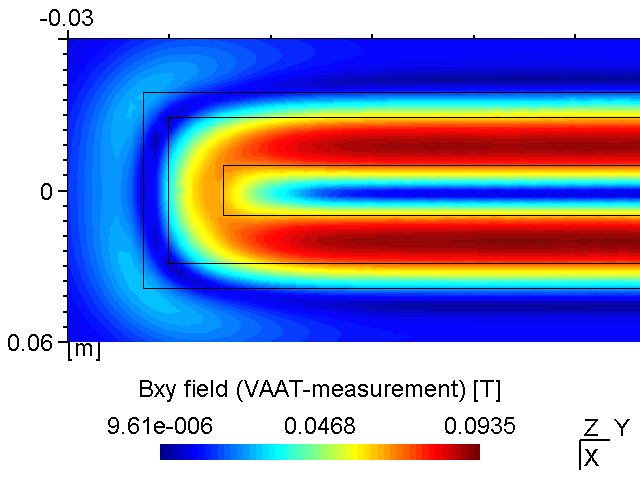
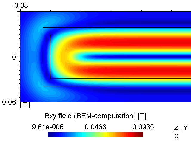
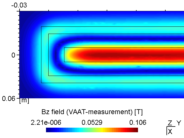
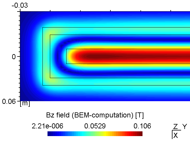
A PK750 magnetron in its strong and standard version has been measured by Von Ardenne Anlagentechnik (VAAT). The BEM compuation is compared with these measurements. The magnets used for the strong magnetron are VACODYM 510 HR from VAC Vakuumschmelze with a remanence of 1.40 T. Additonally we use different permeability values for the yoke material to check the effect of magnetic saturation on the results.
| Parameter | Setting | Unit |
|---|---|---|
| Remanence (strong) | 1.40 | (T) |
| \(\mu_r\)-Vacuum | 1.0 | (-) |
| \(\mu_r\)-Magnets | 1.05 | (-) |
| \(\mu_r\)-Yoke (ST 37 steel) | 1000 | (-) |
| Exemplary PK750 magnetron layout (unbalanced) | FE mesh for numerical field computation (balanced) |
|---|---|
 |
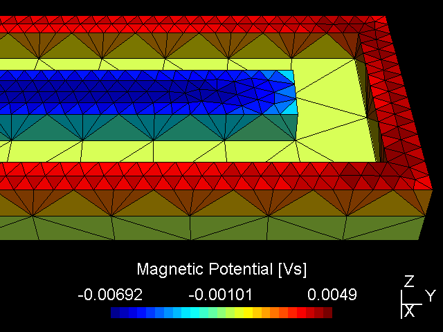 |
While the attached example case and the photograph in Table (tbl:picmc_pk750_modelsetup?) show an unbalanced version of the PK750 magnet assembly, we also did BEM computation and experimental validation with a balanced PK750 version (see mesh file in right graph of Table (tbl:picmc_pk750_modelsetup?)).
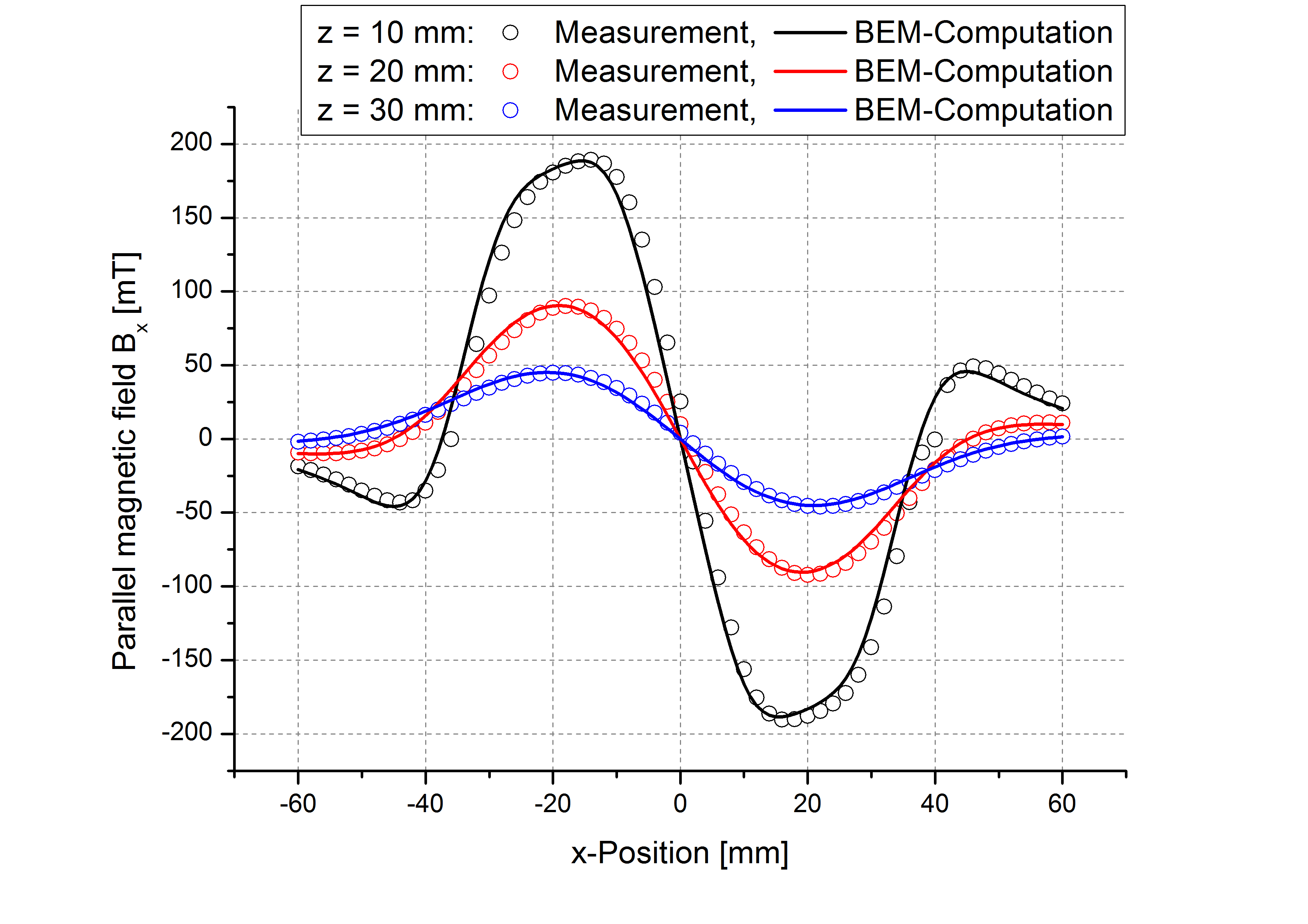
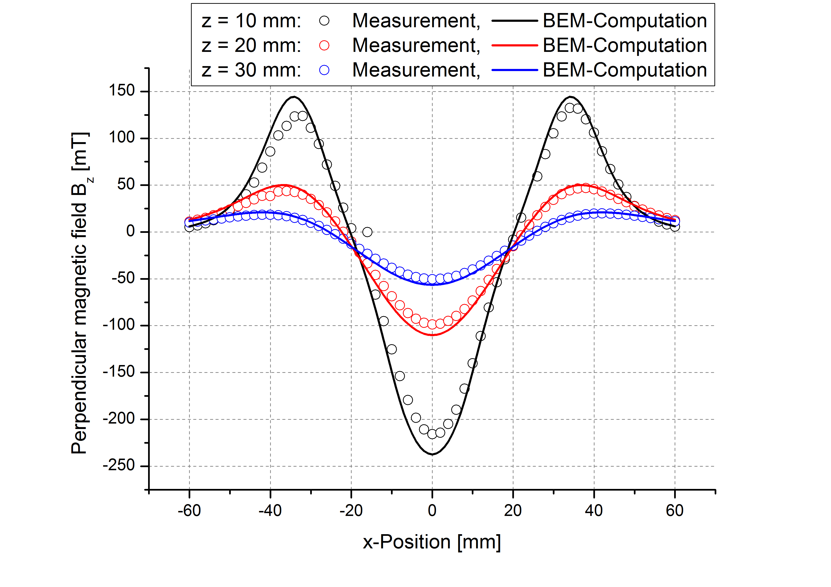
The results are in good agreement with the measurements as seen in the pictures below. Discrepancies should rather be related to remanence deviations of the real magnets.
| \(B_x\) field at z = 10, 20 and 30 mm and y = 400 mm | \(B_z\) field at z = 10, 20 and 30 mm and y = 400 mm |
|---|---|
 |
 |
| Measured \(B_{xy}\) field at z = 20 mm | BEM computed \(B_{xy}\) field at z = 20 mm |
|---|---|
 |
 |
| Measured \(B_z\) field at z = 20 mm | BEM-computed \(B_z\) field at z = 20 mm |
 |
 |
6.2.3 Accuracy issues
6.2.3.1 Using invalid (constant) material parameters
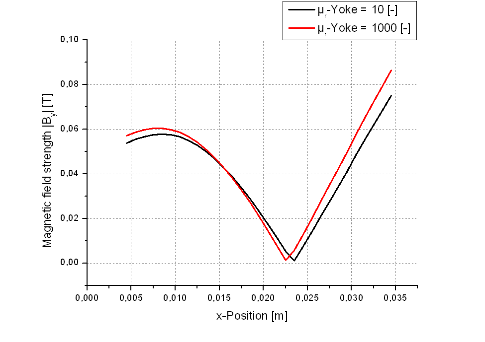
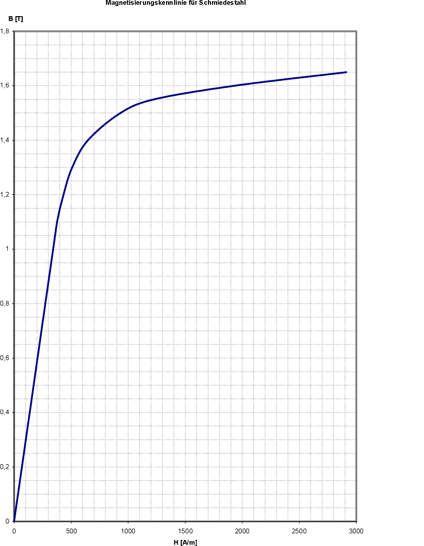
For the materials' magnetic susceptibility we use constant values, e.g. \(\mu_r = 1000\) for ST 37 steel. This approximation is valid as long as the material is beyond magnetic saturation. If this is not the case the effective permeability is somewhere below of the unmagnetized state. This uncertainty can be solved by iterative BEM computation and recalculation of the \(\mu_r\) value according to the material’s hysteresis curve. An automated iterative procedure for that is currently not implemented.
| \(B_y\) field in racetrack zone with \(\mu_r\)-Yoke = 10 and 1000, respectively | Magnetization curve of ST37 steel |
|---|---|
 |
 |
6.2.3.2 Using low mesh resolution
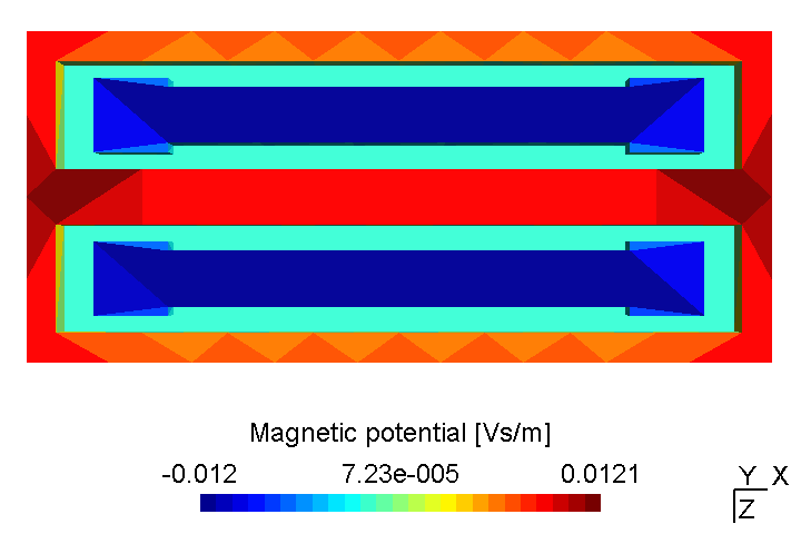
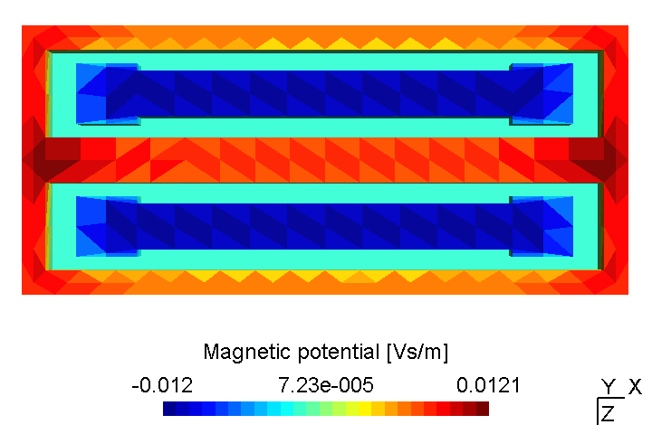
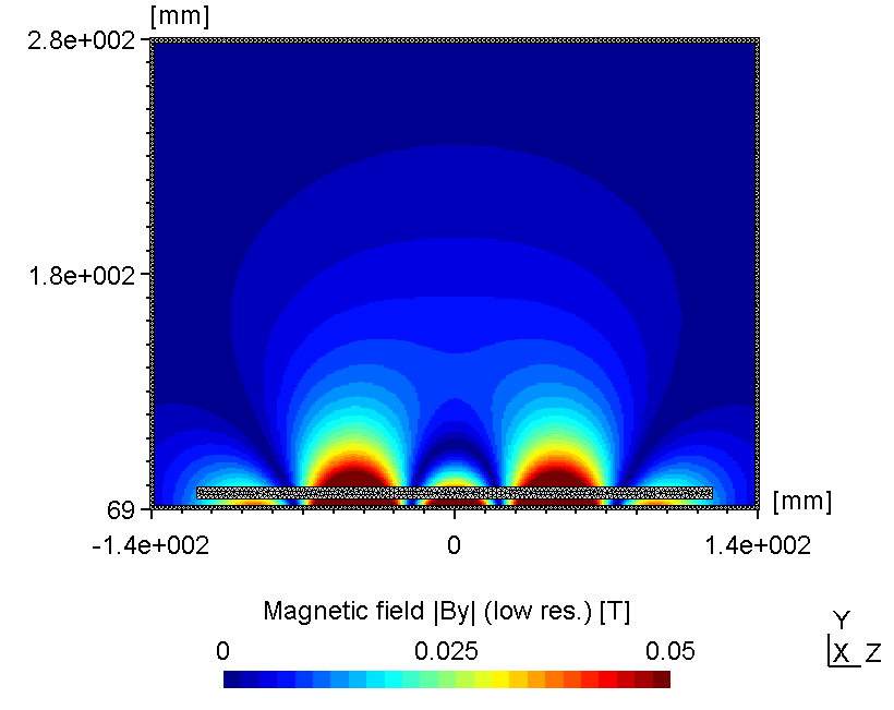
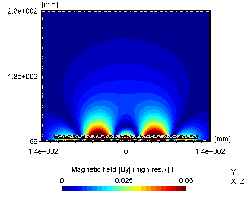
If the region of interest is far away from the mesh, the mesh resolution itself is not crucial for the accuracy of the magnetic field solution. However, as seen below in certain cases the error may be small but not negligible.
| Low mesh resolution | High(er) mesh resolution |
|---|---|
 |
 |
| Low mesh resolution | High(er) mesh resolution |
|---|---|
 |
 |
6.3 2D magnetron discharge
This example shows the setup of a 2D plasma simulation simulation case starting from the GMSH geometry files in a step by step manner. In case you need also information on how to create GMSH geometry files, please check out the DSMC example from section (sec:dsmc_example_1?).
6.3.1 Geometric model
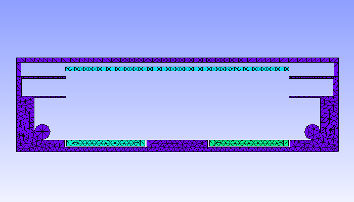
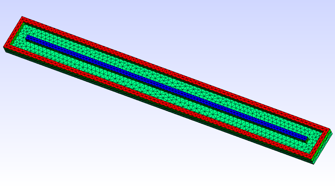
In this example, we simulate a plasma discharge in a dual-magnetron planar sputtering compartment in our Leybold-A700V sputter coater. The rectangular sputter targets are sized \(750\times 88\textrm{ mm}^2\) and are equipped with the unbalanced version of the PK750 magnet assembly (see Tab. (tbl:picmc_a700v?)).
For 2D plasma simulation, a 2D cross-sectional representation of the chamber geometry is used. The chamber geometry still should have a finite thickness in the third direction, which should be in the order of one cell spacing. In contrast, for the magnet, a 3D model is required. After solving the Laplace equation for the magnetic scalar potential on the magnet mesh, the magnetic field is computed in the 2D region of interest within the chamber model. Note: the actual magnet assembly can be located outside of the plasma simulation region, which is also the case in this example.
| 2D-model of a sputter compartment in the Leybold A700V coater | 3D model of the unbalanced PK750 magnet assembly |
|---|---|
 |
 |
The steps to create a complete simulation case out of the geometry files is described in the following.
6.3.2 Step 1: Unpack prepared files
Unzip A700V_PK750.zip into a directory, where the simulation case should be located. The ZIP file contains the GMSH files for the 2D chamber model and the 3D magnet model. The following files are included: * a700v.geo - GMSH model of the 2D chamber compartment * a700v.msh - The same model as *.msh file * pk750-single_standard_unbalanced.geo - 3D GMSH model of the magnet assembly * pk750-single_standard_unbalanced.msh - The same model as *.msh file
6.3.3 Step 2: Create and edit the parameter file
In a plasma simulation with magnetic field computation, two geometric models are required. The chamber geometry defines the region of interest, i.e. the region where the actual plasma simulation takes place. The magnet assembly can be located outside of the region of interest. A new parameter file always has to be generated from the meshed chamber model via the command
$ initpicmc a700vEdit the a700v.par file in an ASCII editor of your choice. First we need to specify useful values for the time interval and time step for plasma simulation:
DT       = 5e-11;
TSIM     = 10e-6;
Set the workmode to plasma simulation:
WORKMODE = 1;We have to adjust the power dissipation:
PSOLL = 10/750;This corresponds to 10 W distributed over 750 mm target length. The 2D cross sectional model has a depth of 1 mm in the third direction, thus, the power has to be scaled by factor 1/750, where 750 mm corresponds to the real length of the sputter target in 3D.
Next step is to specify the list of species treated in the simulation. A minimal set for plasma simulation is a neutral gas molecule, its single charged positive ion and electron. For a plasma in Argon this includes the species Ar, Ar+, and e-:
SPECIES = ["Ar", "Arplus", "e"];The NREAL-parameter is the factor between the number of simulated and real particles and the P0-parameter is the pressure (for neutral particles like Ar) or the initial density (for charged Particles like Ar+ and e-). The appropriate NREAL_Ar-parameter can be calculated from the total pressure and cell spacing (see below). Possible values for the other parameters are:
NREAL_Ar     = 5e9;
P0_Ar        = 0.5;
NREAL_Arplus = 1e5;
P0_Arplus    = 1e13;
NREAL_e      = 1e5;
P0_e         = 1e13;
Depending on what plots you are interested in during the simulation run, insert the species into the appropriate lists in the plotting section:
NUMBER   = ["Arplus", "e"];
DENSITY  = ["Arplus", "e"];
PRESSURE = ["Ar", "Arplus", "e"];
VELOCITY = ["Arplus", "e"];
The unit of the mesh geometry depends on the unit of the coordinates in the meshfile. In our example, the meshfile unit is 1 m, this the value of 1.0 for the UNIT variable is ok. The extent of the bounding box is calculated automatically from the a700v.msh-file, but we have to adjust the cell spacing. The bounding box has a volume of \(360\times 105\times 1\textrm{ mm}^3\). For a plasma density between \(10^{15}\ldots 10^{16}\textrm{ m}^{-3}\), a cell dimension of 1x1x1 mm³ is appropriate. For parallelization, the volume ie divided into 4x3 segments which allows for parallel computation with up to 12 threads.
NX   = [90, 90, 90, 90];
NY   = [35, 35, 35];
NZ   = [1];
Since we have a 2D-xy-model of the sputtering chamber, we have to change the border types in z-direction:
TYPE_z1 = "periodic";
TYPE_z2 = "periodic";
We also want so simulate the magnetic field, so the mesh file for the PK750 magnetron is to be inserted for the BEMMESH variable:
BEMMESH = "pk750-single_standard_unbalanced.msh";Now we need to specify the reactions wich occour on our surfaces. Additionally the wall of the sputtering chamber should be set to ground potential:
Border Wall = {
  vf = "0";
  reactions: {
    add_absorption("Arplus", 1.0);
    add_absorption("e",      1.0);
  };
};
If the simulated substrate should be an insulator instead of a metal, e.g. a glass:
Border Substrate = {
  epsr = 6.0;
  reactions: {
    add_absorption("Arplus", 1.0);
    add_absorption("e",      1.0);
  };
};
The voltage function of the target T1 should be set to "-VP", which is an internal variable. In the actual example the second target is not powered, so it gets the same parameters as the chamber wall:
Border T1 = {
  vf = "-VP";
  reactions: {
    add_plain_reaction("Arplus", 1, 1, ["Ar", "e"], [1, 0.1]);
    set_emission_energy("e", 0, 5, 1);
    add_absorption("e",      1.0);
  };
};

Border T2 = {
  vf = "0";
  reactions: {
    add_absorption("Arplus", 1.0);
    add_absorption("e",      1.0);
  };
};
As mentioned above, the NREAL_Ar-parameter has to be calculated, depending on some other parameters. The number of particles in each cell, has a big impact on the simulation time. A good benchmark are ca. 20 simulated particles/cell. Depending on the Ar pressure (P0_Ar = 0.5 Pa), temperature (T0 = 300 K) and the cell dimension (1x1x1 mm³) you can calculate the number of real particles per cell and then adjust the NREAL_Ar:
\[N = \frac{pV}{kT} = 1.21\times 10^{11}\textrm{ particles/cell} \Rightarrow \textrm{NREAL\_Ar} = 5\times 10^{9} \Rightarrow \textrm{24 simulation particels/cell}\]
6.3.4 Step 3: Create and edit the magnetic template
Create a template for the magnetic fieldsolver:
$ initbfield a700vEdit the a700v.bem-file. The relative permeabilities of the three domains (vacuum, magnets and yoke) can stay as suggested by the default values:
Domains = [1, 1.05, 1000];Next, the polarity of all physical surfaces and their relation and belonging to magnetic domains has to be specified. The val-parameter is the magnetic remanence value. The domain- and neighbourdomain-parameter correspond to the above defined domains numbers. Please note that the domain numbering scheme starts at 0, not at 1. The bottom of the inner and outer magnet are connected to the yoke and all other surfaces are connected to vacuum:
Boundary Outer_Magnet_Top    = {icodec = 1; type = "interface"; val = -1.40;  domain = 1; neighbourdomain = 0;};
Boundary Outer_Magnet_Bottom = {icodec = 2; type = "interface"; val =  1.40;  domain = 1; neighbourdomain = 2;};
Boundary Inner_Magnet_Top    = {icodec = 3; type = "interface"; val =  1.40;  domain = 1; neighbourdomain = 0;};
Boundary Inner_Magnet_Bottom = {icodec = 4; type = "interface"; val = -1.40;  domain = 1; neighbourdomain = 2;};
Boundary Magnet_Skin         = {icodec = 5; type = "interface"; val =     0;  domain = 1; neighbourdomain = 0;};
Boundary Yoke                = {icodec = 6; type = "interface"; val =     0;  domain = 2; neighbourdomain = 0;};
A complete version of the model including both parameter files can be found here.
6.3.5 Step 4: Start magnetic field computation
Start the computation with n processes. In our case with n = 12 just enter:
$ rvmmpi -bem 12 a700vFor magnetic field computation the number of parallel processes does not have to match with the number of segments, even a higher number of parallel processes can be used.
Check out the output for the following lines:
MASTER <- {BEM 10}:     [MESSAGE]        domain:   2 checksum:  1.0319e-13
MASTER <- {BEM  6}:     [MESSAGE]        domain:   1 checksum: -5.0333e-13
MASTER <- {BEM  1}:     [MESSAGE]        domain:   0 checksum:  1.2566e+01
For all areas the sum should be exactly \(4\pi = 12.5664\) or \(0\) (round-off errors like 1e-12 are ok).
6.3.6 Step 5: Start simulation
Start the simulation with n processes (n may not exceed the number of subvolumes). In our case with n = 12 just enter:
$ rvmmpi -picmc 12 a700vIn the following a few typical results for different substrate and magnet parameters are presented.
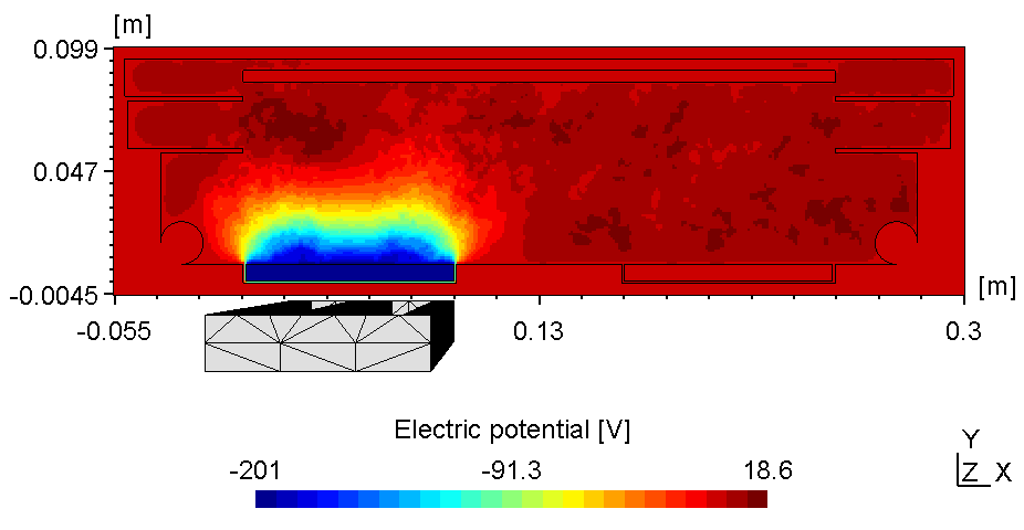
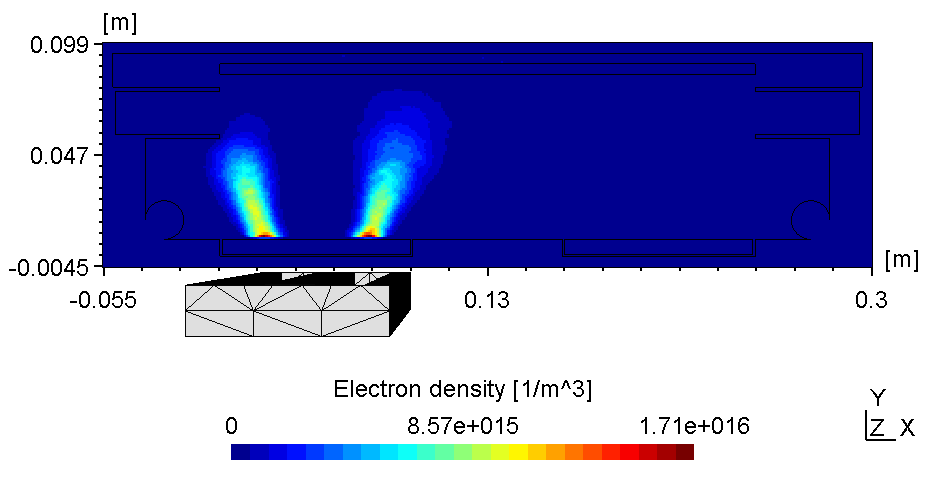
6.3.7 Substrate on ground potential
The plasma in a 2D set-up is not coupled and thus, more sensitive to the anode configuration. With the substrate on ground potentialthe right plasma is as bright as the left one (see figure 1).
| Electric potential | Electron Density |
|---|---|
 |
 |
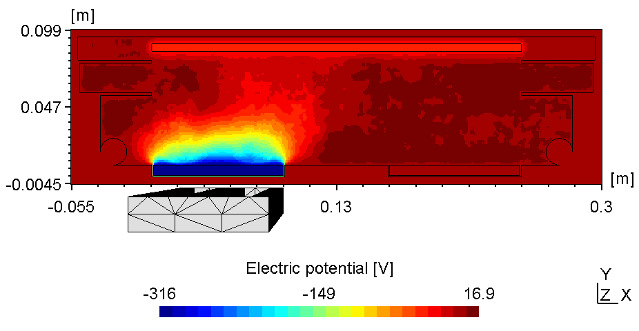
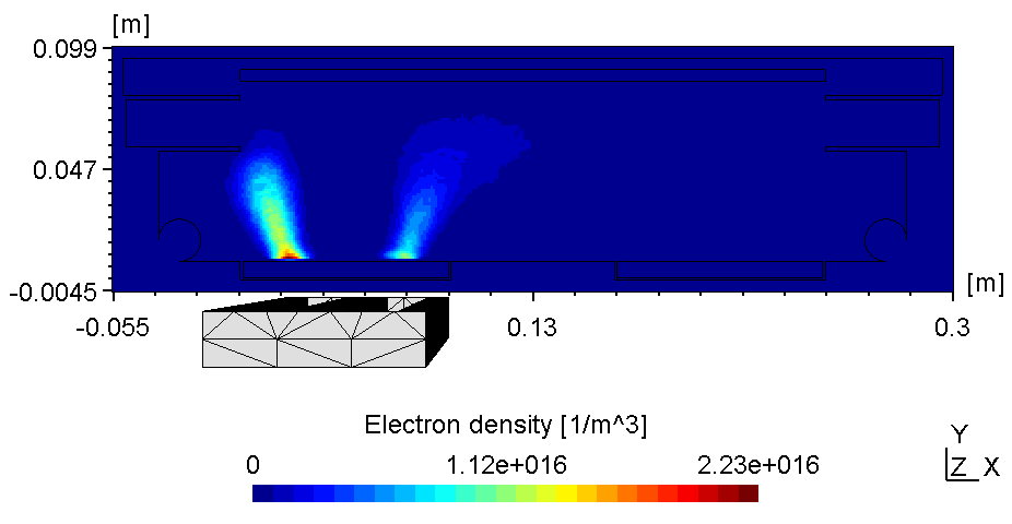
6.3.8 Substrate on floating potential
Here the left plasma is conductively connected to the ajacent chamber wall, the right one however is connected with the top of the chamber wall. Thus, with the substrate on floating potential some of the anodic surface is shielded causing the right plasma to fade (see figure 2). Due to the uncoupled electron drift current in a 2d setup this effect is even more pronounced. Thus, if using constant power the voltage can drop below ignition point causing the right plasma to diminish.
| Electric potential | Electron Density |
|---|---|
 |
 |