DSMC and PICMC documentation

3.1.1 Simple scalar cut-plane

One of the easiest and most frequent tasks is to create a quick cut-plane aligned parallel to XY, XZ or YZ plane. Assumed, we have the file pressure_Ar_60.00ms.pos from a DSMC run of the tube example as output file, and would like to have a scalar pressure plot in the XY plane. The according script - let's call it extract.r looks like follows:

compiletime load "module_ppp.so";
case = BATCH.file;
time = 60;
PPP obj = {};

obj.read("$case/pressure/pressure_Ar_$(time%,2f)ms.pos", "pAr");
obj.xy_plane(0, 10, "nearest_neighbour");
obj.write_pos_scalar_binary("extract/$case-pressure_xy.pos", 
                            "Ar pressure [Pa]", pAr);

In order to run this script with rvm, a subfolder extract should be in place. An example session is shown in the following, it assumes that the simulation parameter file is named tube.par and the post processing script is cutplane.r.

ap@sim159:~/sim/examples/ex1-tubeflow$ rvm -b cutplane.r tube
Created View {pAr}
File tube/pressure/pressure_Ar_60.00ms.pos has 96000 scalar and 0 vector points
XY-Plane extract, z0 = 0 +/- 10, method = 'nearest_neighbour'
Writing 'Ar pressure [Pa]' into scalar file 'extract/tube-pressure_xy.pos' 
(2400 of 2400 points)

As result, the output file extract/tube-pressure_xy.pos is created and can be viewed in GMSH.

The meaning of the commands in the last three lines is as follows:

• obj.read("input.pos", "variable_name");
  • The first parameter is the filename of the binary POS file
  • The expression $(time%,2f) will be replaced by the value of the variable time with 2 digits, i.e. 60.00.
  • The second parameter is a variable name used for referencing these data in a later step
• obj.xy_plane(0, 10, "nearest_neighbour");
  • Create a cutplane parallel to the XY coordinates and positioned around z=0 (first parameter)
  • Consider each point in a search radius \(z = 0 \pm 10\) on both sides of the cutplane and
  • Display the nearest point onto the cutplane
• obj.write_pos_scalar_binary("output.pos", "plot_title", expression);
  • This writes a scalar output file named "output.pos".
  • The "plot_title" will be shown as view title in GMSH.
  • With expression the scalar output value can be specified. In the above example, it is just the pressure value named pAr.

Besides of obj.xy_plane(z0, delta_z, "method") there are also obj.xz_plane(y0, delta_y, "method"); and obj.yz_plane(x0, delta_x, "method"); available.

3.1.2 Scalar cut-plane with arithmetics

Within the expression parameter it is possible to do some arithmetics. If e.g. the pressure should be plotted in mTorr instead of Pa (1 mTorr = 133 mPa), the following script will do it:

compiletime load "module_ppp.so";
case = BATCH.file;
time = 60;
PPP obj = {};

obj.read("$case/pressure/pressure_Ar_$(time%,2f)ms.pos", "pAr");
obj.xy_plane(0, 10, "nearest_neighbour");
obj.write_pos_scalar_binary("extract/$case-pressure_xy.pos", 
                            "Ar pressure [mTorr]", pAr*1000/133);

3.1.3 Scalar cut-plane with triangulation

By replacing the command write_pos_scalar_binary by write_pos_triangulate it is possible to create a triangulated scalar view:

compiletime load "module_ppp.so";
case = BATCH.file;
time = 60;
PPP obj = {};

obj.read("$case/pressure/pressure_Ar_$(time%,2f)ms.pos", "pAr");
obj.xy_plane(0, 10, "nearest_neighbour");
obj.write_pos_triangulate("extract/$case-pressure_xy.pos", 
                            "Ar pressure [mTorr]", pAr*1000/133);

3.1.4 Scalar cut-plane from multiple input files

Let’s assume we would like to plot the flux (=density*velocity) in positive X direction and have the density as well as the number plots activated. Arithmetics in the postprocessing script allow to compute the density from the particle number and from that the flux:

compiletime load "module_ppp.so";
case = BATCH.file;
time = 60;
PPP obj = {};

obj.read("$case/number/number_Ar_$(time%,2f)ms.pos", "N");
obj.read("$case/velocity/velocity_Ar_$(time%,2f)ms.pos", "v");
obj.read("$case/cell_volumes.pos", "vol");
obj.xy_plane(0, 10, "nearest_neighbour");
obj.write_pos_triangulate("extract/$case-xflux_xy.pos", 
                          "Ar flux [1/m^2s]", 
                          vol>0 ? 8e12*N/vol*v_x ! 0);

The velocity is a vector plot; thus, by reading in the velocity with variable name v, the three vector components v_x, v_y, v_z are internally created and can be used in the expression arithmetics. The density is computed from the number N as 8e12*N/vol, where 8e12 is the scaling factor NREAL_Ar between real and simulated number of Ar atoms. However, for some simulation cells, which are fully contained within a wall of the geometric model, the volume vol is zero and thus, the above expression will fail. Therefore, the expression for the density contains an implitic if statement in the form vol>0 ? ... ! .... The expression after the ? is taken, if vol>0 holds, otherwise the expression after the ! is computed instead.

Depending on the statistics, the cut-plane of the flux plot may look a bit noisy. In this case, it helps to use the "interpolate" option rather than "nearest_neighbour":

Table 3.1: Cutplanes obtained with the nearest_neighbour and the interpolate method

obj.xy_plane(0, 10, "nearest_neighbour");	obj.xy_plane(0, 10, "interpolate");

Putting all the arithmetics into the expression argument can get confusing. There are multiple ways to define the density expression separately, one method is to define it within the PPP object:

compiletime load "module_ppp.so";
case = BATCH.file;
time = 60;
PPP obj = {
  float NREAL = 8e12;
  float nAr: vol>0 ? NREAL*N/vol ! 0;
};

obj.read("$case/number/number_Ar_$(time%,2f)ms.pos", "N");
obj.read("$case/velocity/velocity_Ar_$(time%,2f)ms.pos", "v");
obj.read("$case/cell_volumes.pos", "vol");
obj.xy_plane(0, 10, "nearest_neighbour");
obj.write_pos_triangulate("extract/$case-xflux_xy.pos", 
                          "Ar flux [1/m^2s]", nAr*v_x);

Since the variables N and vol are not known during definition of nAr within the PPP object, it is important to use the alias method (i. e. the ":") instead of the assign method (i. e. "=") for definining density. The result of this modified script is the same as for the script above but now, it looks more clearly arranged.

Another way is to create an input data set of the density via the create_scalar method:

compiletime load "module_ppp.so";
case = BATCH.file;
time = 60;
PPP obj = { };

obj.read("$case/number/number_Ar_$(time%,2f)ms.pos", "N");
obj.read("$case/velocity/velocity_Ar_$(time%,2f)ms.pos", "v");
obj.read("$case/cell_volumes.pos", "vol");

obj.create_scalar("nAr", vol>0 ? 8e12*N/vol ! 0);

obj.xy_plane(0, 10, "nearest_neighbour");
obj.write_pos_triangulate("extract/$case-xflux_xy.pos", 
                          "Ar flux [1/m^2s]", nAr*v_x);

3.1.5 Time averaging

In order to perform averaging of the same quantity over several time steps, it is sufficient to call the function obj.read(...) several times but with the same variable name. An example is given in the following:

compiletime load "module_ppp.so";
case = BATCH.file;
T1 = 100; T2 = 200; DT = 10;
time = 60;
PPP obj = {
  float NREAL = 8e12;
  float nAr: vol>0 ? NREAL*N/vol ! 0;
};

for (time=T1; time<=T2; time=time+DT) {
  obj.read("$case/density_Ar_$(time%,2f)ms.pos", "d");
  obj.read("$case/velocity_Ar_$(time%,2f)ms.pos", "v");
}
obj.read("$case/cell_volumes.pos", "vol");
obj.xy_plane(0, 10, "nearest_neighbour");
obj.write_pos_triangulate("extract/$case-xflux_xy.pos", 
                          "Ar flux [1/m^2s]", nAr*v_x);

The read command of the PPP object automatically recognizes if one variable is used several times and performs an averaging of the data in this case.

3.1.6 Development over time

If you would like to illustrate the development of the same quantity over several time steps, you need to call obj.append(...) several times but with the same variable name and then one of the write_pos_time_steps functions. An example is given in the following:

compiletime load "module_ppp.so";
compiletime load "module_system_linux.so";

# defining parameters
case   = BATCH.file;
start  = 100;
end    = 200;
dtime  = 20;
unit   = "us";
z      = 0;
folder = "density";
files  = "density_e";

# create ppp subfolder if it does not exist
System FS = { rootpath = "$case"; };
if (FS.folder_exists("ppp") == 0) then {
  out "Creating folder $case/ppp\n";
  FS.create_folder("ppp", 493)
};

# applying a cut plane to each time step
for (time=$start; time<=$end+0.001; time=time+dtime) {
  PPP obj1 = {};

  obj1.read("$case/$folder/$(files)_$(time% 4,2f)$(unit).pos", "X");
  obj1.xy_plane($z, 10, "nearest_neighbour");
  obj1.write_pos_scalar_binary("$case/ppp/cut_$(files)_$(time% 4,2f)$(unit).pos", 
                               "$files", X);
}

# appending the cut planes to each other
PPP obj2 = {};
for (time=$start; time<=$end+0.001; time=time+dtime) {
  obj2.append("$case/ppp/cut_$(files)_$(time% 4,2f)$(unit).pos", "Y");
}
obj2.write_pos_time_steps_scalar_binary(
  "$case/timestep_cut_$(z)mm_$(files)_$(start)-$(end)$(unit).pos", "$files", "Y"
);

First of all module_system_linux.so is loaded, which is needed for creating the ppp subfolder for storing the intermediate cut planes. Next some parameters are set including the time interval, the z position of the cut plane and the name of the plot. Then the ppp subfolder is created, where the cut planes generated in the next part are stored. In the last part these cut planes are appeded to each other and written to the output file.

The order of first creating the cut planes and then appending them to each other is important, because it is (at the moment) not possible to make cut planes of variables with multiple time steps. Additionally the write_pos_time_steps functions can only be called on the variable name and not on an expression, so that calculations have to be done before.

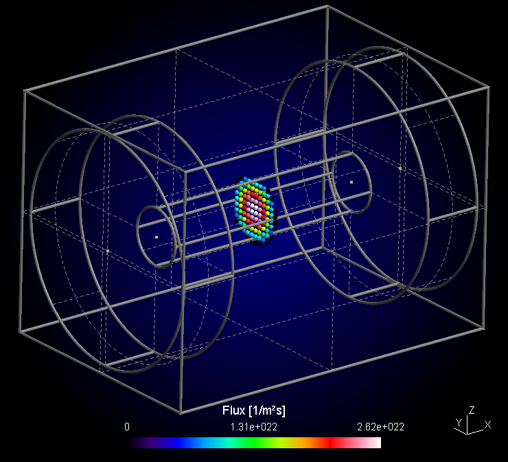
3.1.7 Generating vector plots as cut plane

Finally we would like to plot the flux as vector plot. All we have to do is to replace the obj.write_pos_scalar(...) by obj.write_pos_vector(...). Since a vector plot has three components, we have three instead of one expression arguments.

compiletime load "module_ppp.so";
case = BATCH.file;
time = 60;

PPP obj = {
  float NREAL=8e12;
  float density: vol>0 ? NREAL*N/vol ! 0;
};

obj.read("$case/number/number_Ar_$(time%,2f)ms.pos", "N");
obj.read("$case/velocity/velocity_Ar_$(time%,2f)ms.pos", "v");
obj.read("$case/cell_volumes.pos", "vol");
obj.xy_plane(0, 20, "interpolate");
obj.write_pos_vector("extract/$(case)-cutplane_xy.pos", "Flux (1/m^2 s)", 
                     density*v_x, density*v_y, density*v_z);

3.1.8 Revert POS file data to original state

The obj.identity() function enforces to transfer the whole input data into the view data. It is only necessary to invoke this function, if the view data are reduced due to a previous data operation such as a cutplane. Without data operation, obj.identity() is internally invoked, automatically.

compiletime load "module_ppp.so";
case = BATCH.file;
time = 60;
  
PPP obj = {};
  
obj.read("$case/number/number_Ar_$(time%,2f)ms.pos", "N");
obj.xy_plane(0, 10, "nearest_neighbour");
obj.write_pos_scalar("cutplane_xy.pos", "Ar number [#]", N);
obj.identity();
obj.read("cell_volumes.pos", "vol");
obj.write_pos_scalar("density_Ar.pos", "Ar density [#/m^3]", vol>0 ? N/vol ! 0);

3.1.9 General (oblique) interpolation views

For cutplanes which are not parallel to one of the coordinate planes, it is possible to specify them in a more general way. For this purpose, a general description of a parametric plane looks as follows:

\[\vec{r}(s,t) = \vec{x}_0 + s\left(\vec{x}_1-\vec{x}_0\right) + t\left(\vec{x}_2-\vec{x}_0\right)\](3.1)

The accordant post processing command is written as:

obj.plane(x0, y0, z0,  x1, y1, z1,  x2, y2, z2,  delta, N, M, "method");

First, the three points of the above equation are given coordinate-wise (i.e. the first 9 parameters). The next parameter delta is the vertical distance to the plane, wherin points are considered for interpolation. The integer numbers N, M give the resolution of the cut plane in direction of the first and second vector. Update: It is possible to specify 0, 0 for N, M; in this case the actual resolution of the imported POS file will be taken.

An example of an oblique plane with respect to our tube DSMC case is shown in the following:

compiletime load "module_ppp.so";
case = BATCH.file;
time = 60;

PPP obj={
  float density: vol>0 ? N/vol ! 0;
};

obj.read("$case/number/number_Ar_$(time%,2f)ms.pos", "N");
obj.read("cell_volumes.pos", "vol");

obj.plane(-110, -210, -210,  200, 210, 0,  200, -210, 0,  
          15,  40, 40, "interpolate");

obj.write_pos_scalar_binary("extract/$case-obliqueplane.pos", 
                            "Density [1/m^2 s]", density);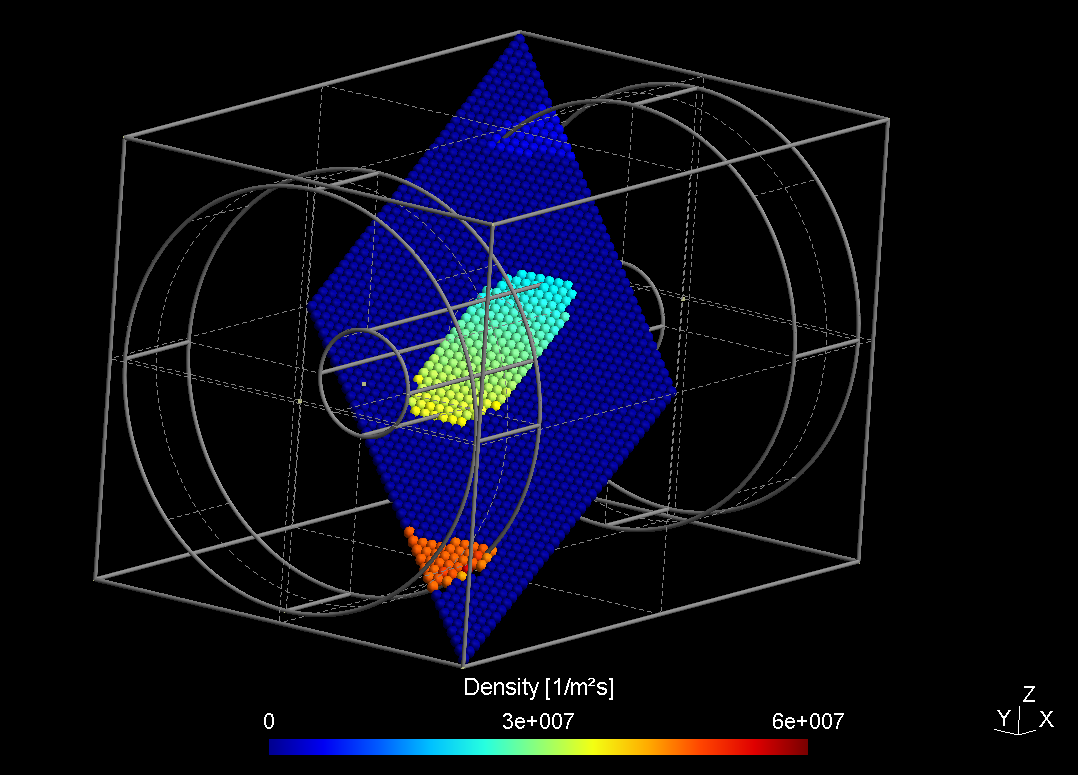

Analogously, it is possible to extract data along a straight line:

\[\vec{r}(s) = \vec{x}_0 + s\left(\vec{x}_1-\vec{x}_0\right)\](3.2)

with the postprocessing command:

obj.line(x0, y0, z0,   x1, y1, z1,    delta, N, "method");

3.1.10 Additional output formats

obj.write_vtk_scalar("output.vtp", "View title", expression);
obj.write_vtk_vector("output.vtp", "View title", expression_x, expression_y, expression_z);

obj.write_tec_scalar("output.dat", "View title", expression);
obj.write_tec_vector("output.dat", "View title", expression_x, expression_y, expression_z);

obj.write_txt("file_name.txt", ["col1", "col2", ...], [exp1, exp2, ...]);

compiletime load "module_ppp.so";

PPP obj1 = {};

obj1.read("absorption.pos", "A");
obj1.xy_plane(-141.75, 10, "nearest_neighbour");
obj1.write_pos_scalar_binary("absorption-2D.pos", "SiH4 absorption [1/m^2 s]", A);

PPP obj2 = {};

obj2.read("absorption-2D.pos", "A");
obj2.line(420, -380, -141.75,   607.5, -380, -141.75,  40, 19, "average");
obj2.write_txt("profile_avg.txt", 
               ["r [mm]", "abs [1/m^2 s]", "abs [%]"], 
               [x-420, A, 100*A/A_max]);

         r [mm]   abs [1/m^2s]        abs [%]

        4.93421    3.80416e+20        99.9454
        14.8026    3.77636e+20        99.2152
        24.6711    3.80623e+20            100
        34.5395     3.7374e+20        98.1916
        44.4079    3.75455e+20         98.642
        54.2763    3.73143e+20        98.0347
        64.1447    3.68571e+20        96.8336
        74.0132    3.63662e+20        95.5439
        83.8816    3.58961e+20        94.3087
          93.75    3.54935e+20         93.251
        103.618    3.47403e+20         91.272
        113.487    3.43792e+20        90.3235
        123.355    3.31429e+20        87.0752
        133.224    3.24909e+20        85.3624
        143.092    3.18416e+20        83.6563
        152.961    3.03792e+20        79.8144
        162.829    2.88857e+20        75.8905
        172.697    2.66338e+20        69.9741
        182.566    2.29174e+20        60.2102

obj.write_csv("file_name.csv", ["col1", "col2", ...], [exp1, exp2, ...]);

3.1.11 Numerical integration

The numerical integration feature is currently available for cut-planes only. In our tube example we might want to integrate the particle flux through the tube. This can be accomplished as follows:

compiletime load "module_ppp.so";

mesh_unit=1e-3;
Nsccm = 4.478e17;

file "integration.txt" << for (time=20; time<=400; time=time+20) {
  PPP obj={};
  obj.read("density_Ar_$(time).00ms.pos", "density");
  obj.read("velocity_Ar_$(time).00ms.pos", "v");
  obj.plane(200, -60, -60,   200, 60, -60,   200, -60, 60,  
            10, 0, 0, "interpolate");
  flow = obj.integrate(density*v_x)*mesh_unit^2/Nsccm;
  out "$(time)  $(flow)\n";
}

In the script shown above, the density and velocity of Argon are loaded for a complete time series t=20...400 ms. For each time step, a PPP object is created, and the flux is generated via the expression density*v_x within the cut plane. With the integrate function, the total flux through the tube cross section can be computed.

The numerical integration is internally performed over triangles of adjacent points. For each triangle, the average of the three point values is multiplied with the area of the triangle element. If the mesh unit is not 1 m, the integration result should be multiplied with mesh_unit^2 in order to get the correct unit.

In the example script, the result is additionally divided by the particle number per second for 1 sccm in order to get the flow in sccm.

3.1.12 Merging of (position) plots

In the normal output files (e.g. density) each point corresponds to a single cell with its position and its value. A second density plot has the same cells at the same position but with different values. Therefore it makes no sense to merge these files into a single one, this is only the case for position plots, where the positions of particles are stored independent of the cell resolution. By merging multiple of these files the illustration of the particle movement is possible:

compiletime load "module_ppp.so";

PPP obj = {};

for (float time=0; time<=100; time=time+0.5) {
  obj.merge("position/position_e_$(time %,2f)ns.pos", "pos");
 }
obj.write_pos_scalar_binary("position_e_0-100ns.pos", "e position", pos);

In this example a position plot each 0.5 ns for a time interval between 0 and 100 ns is merged and written to a single file. The syntax of the merge function is identical to that of the read function.