
DSMC and PICMC documentation
2022-04-20
2.1 Parameter file review
This site explains step by step all parts of the parameter file.
2.1.1 General parameters
DT       = 1e-5;
TSIM     = 1.0;
DT is the time step in [s] of the simulation. For DSMC its usually in the order of 10-6-10-5 and all particles are moved in each time step. In PICMC mode its in the order of 10-12-10-10 and only electrons are moved in each time step. The ions and neutral atoms are moved appr. each 30th and 300th step depending on the mass ratio related to the electrons. The value should be chosen in a way that the mean travelling distance of particles is less than their mean free path.
Example: If we assume Argon (Ar) as gas species and a mean total pressure of about 0.5 Pa, then the mean free path of the gas atoms will be about 1.3 cm (see mean free path, section (sec:num_constraints_dsmc?)). At 300 K, the mean velocity of an Ar atom is 398 m/s. Within a time step of 10-5 s this yields a mean travelling distance per time step of about 4 mm.
TSIM gives the total simulation time in [s] and is in the order of 1 for DSMC and 10-5 for PICMC.
NPLOTS   = 10;
NDUMPS   = 1;
NPLOTS gives the total number of plot evenly distributed over the total simulation time. If you make a restart of a simulation the number of plots made before is not taken into account.
The value NDUMPS is the number of particle dumps / checkpoints made during the simulation also evenly distributed over the total simulation time. If you have a checkpoint you can continue / restart the simulation from that point on. A new checkpoint overwrites the old one. A value of 1 means that the checkpoint is created when the simulation reaches its end. It is recommended to increase this value if the simulation is very time-consuming and you would lose several days if your simulation unexpectedly crashes.
WORKMODE = 0;
PSOLL    = 1;
PSAMPLE  = 1e-7;
WORKMODE accepts three different values, 0 if you want to simulate the gasflow of neutral particles with the DSMC method, 1 if a PICMC plasma simulation is favored or 2 if you are only interested in the electric field of a given setup. In case of a PICMC simulation the next two parameters are likewise evaluated. PSOLL is the aimed power dissipation in [W] and PSAMPLE is the sampling time for this power setpoint in [s].
T0       = 300;
NCOUNTS  = 100;
VPMAX    = 1000;
The T0 parameter defines the initial particle and border temperature in [K]. You could also use a non-trivial temperature distribution on a wall. NCOUNTS is the number of sampling intervals for particle counters. The value of VPMAX is the maximum voltage which is used in the voltage function.
2.1.2 Species
SPECIES      = ["Ar", "Arplus", "e"];
NREAL_Ar     = 1e12;
P0_Ar        = 0.5;
NREAL_Arplus = 1e5;
P0_Arplus    = 1e14;
NREAL_e      = 1e5;
P0_e         = 1e14;
The selection of gas species is defined within an array SPECIES. If multiple species are required, they can be written in a comma separated list such as above. A list of all available species can be found in section (sec:prep_species_list?). For each species SP, the parameters NREAL_SP and P0_SP must be defined with the following meaning:
NREAL_SP: Statistical weight of the speciesSP. A value of e.g. 1e12 means, that one particle in the simulation corresponds to 1e12 particles in the physical reality. The collision statistics are handled according to this weighting factor. It is possible to use different weighting factors for different species; e.g. if we have 1 % oxygen diluted in Argon, we may useNREAL_Ar = 1e12; NREAL_O2 = 1e10;in order to get a similar amount of simulation particles for both species.P0_SP: IfSPis a neutral species, this defines the initial pressure in Pa. IfSPis a charged species (electron / ion), the initial density in [1/m³] is expected here instead.
In order to define proper values for these parameters, some statistical constraints of your simulation case have to be taken into account first. Please refer to the section (sec:num_constraints_dsmc?) for general information.
2.1.3 Frozen species
On demand, some of the species contained in the SPECIES array can be treated as frozen. In this case, no particles are stored; instead the species are treated as continuous background. Species properties considered are then averaged values of density, velocity components <vx>, <vy>, <vz> as well as the square velocity <v2>. The averaged values are stored cell-wise. In case of initialization of a frozen species via the P0_species parameter in the parameter file, only the averaged density and the square velocity will be non-zero. An alternative is to load the species from a checkpoint of another simulation. In this case, also the flow velocity stored in <vx>, <vy>, <vz> can be relevant.
Example: In a PIC-MC plasma simulation in Argon, the Argon background should be treated as continuous, homogeneous background. In this case, the species definition section in the parameter file could look as follows.`SPECIES = [“Ar,” “Arplus,” “e”];
NREAL_Ar     = 6e+9;
P0_Ar        = 0.5;
NREAL_e      = 20000;
P0_e         = 1e13;
NREAL_Arplus = 20000;
P0_Arplus    = 1e13;

FROZEN_SPECIES = ["Ar"];
Note: If charged species (electrons, ions) are present in a DSMC simulation (WORKMODE=0), they are automatically being treated as frozen.
2.1.4 Plots
NUMBER      = ["Ar", "Arplus", "e"];
DENSITY     = ["Arplus", "e"];
PRESSURE    = [];
TEMPERATURE = [];
ENERGY      = ["Arplus", "e"];
VELOCITY    = [];
COLLISION   = [];
ABSORPTION  = ["Arplus", "e"];
DESORPTION  = [];
MESHDATA    = [];

POSITION    = [];

FIELD       = ["PHI"];

COVERAGE    = [];
DEPOSITION  = [];
Here, we have some predefined lists for each output quantity, where the species of interest can be inserted. Please refer to section (sec:post_processing_data?) for further details.
Depending on your choice, the respectively quantity will be dumped into a 3D-outputfile for each plot interval (defined by TSIM and NPLOTS). The 3D-outputfiles have the ending .pos and can be displayed with GMSH. They can be further postprocessed via the RIG-VM postprocessing module in section (sec:ppp_rvm?) or via GMSH (section (sec:ppp_gmsh?)).
2.1.5 Simulation volume
UNIT = 1.0;
BB   = [x0, y0, z0, x1, y1, z1];
The standard treatment of the simulation volume is to put the whole geometric mesh model within a rectangular box, which is referred to as Bounding box. The bounding box dimensions are defined within the vector BB, where, (x0, y0, z0) and (x1, y1, z1) specify two opposing edges with lower and upper coordinates. Important: Before specifying any coordinates, first make sure that the UNIT variable correctly represents the scale of your geometric model:
| Mesh unit | UNIT variable |
|---|---|
| m | 1.0 |
| mm | 0.001 |
| inch | 0.0254 |
When the parameter file is created via initpicmc meshfile the upper and lower edge coordinates are automatically set according to the maximum / minimum node coordinates occurring in the mesh file. However it is principally possible to set different bounding box dimensions e.g. in order to perform the simulation in only a fraction of the geometric model.
After you have set the bounding box dimensions, the simulation volume can be divided into multiple segments via the vectors NX, NY, NZ, and the number of cells for each segment can be specified. In the 2D plasma example in section (sec:picmc_2d_a700v?) the size of the bounding box is 360 mm in X, 105 mm in Y and 1 mm in Z direction. Assumed the cell dimension should be 1x1x1 mm³, we would need 360x105x1 cells. A possible segmentation would be:
NX = [60, 60, 60, 60, 60, 60];
NY = [35, 35, 35];
NZ = [1];
This gives six segments in X direction with 60 cells each, i.e. 360 cells in total, while the total number of cells in Y direction is 3x35 = 105. As it is a 2D model within the XY plane, there is no variation in Z direction expected; therefore the number of cells in Z is 1. The above shown segmentation gives a total of 18 segments, i.e. up to 18 CPUs can be used for parallel execution of the job.
Without further parameters the segmentation is always equi-distant. In order to provide a segmentation with customized distances, the vectors DIV_X, DIV_Y, DIV_Z can be used.
DIV_X = [lx1, lx2];
DIV_Y = [ly1, ly2];
DIV_Z = [lz1, lz2];
The length values of the segments in the respective direction have to be in the scale given by the UNIT parameter above. The number of entries in DIV_X and NX etc. must fit and the sum of the segment lengths (lx1+lx2+...+lxn) has to be equal to the corresponding bounding box length.
TYPE_x1 = "outlet";
TYPE_x2 = "outlet";
TYPE_y1 = "outlet";
TYPE_y2 = "outlet";
TYPE_z1 = "outlet";
TYPE_z2 = "outlet";
Finally, it must be defined what happens if a particle crosses the outer boundary of the bounding box. The bounding box has six sides labeled x1, x2, y1, y2, z1, z2 (i.e. lower x side, upper x side etc.). For each side, the type can be one of the following:
"outlet": Particles hitting this surface disappear immediately."specular": Particles are specularly reflected."periodic": Particles crossing this border are re-inserted at the opposite surface.
2.1.6 Manually segmented simulation domain
block MQUAD: {
  block FirstBox: {
    DIV_X = [50, 50];
    DIV_Y = [100];
    DIV_Z = [20];
    NX = [5, 5];
    NY = [10];
    NZ = [2];
    X0 = 0; Y0 = 0; Z0 = 0;
  };
  block SecondBox: {
    DIV_X = [50, 50];
    DIV_Y = [100];
    DIV_Z = [20];
    NX = [5, 5];
    NY = [10];
    NZ = [2];
    NREAL_SCALE_X = [0.5, 1.0];
  };
};

block MJOIN: {
  FirstBox.join_center(SecondBox, "x");
};
For some geometric models a common rectangular simulation box is not efficient since large parts of the simulation volume might be unused. In such case it is possible to use the Multiquad approach, where multiple bounding boxes with individual segmentation and cell spacing can be defined for different parts of the simulation model.
As shown above, this is done by defining several segmented bounding boxes within a construct block name = { ... }. Each name must start with a letter and can additionally contain digits or the _ underline character. A box must contain the three vectors DIV_X, DIV_Y, DIV_Z, which contain the dimensions of the respective segments in x, y, and z direction. Additionally, the vectors NX, NY, NZ contain the number of cells for each segment. Optionally, the following additional parameters can be included:
NREAL_SCALE= global parameter to scale theNRealvalue for each species within this boxNREAL_SCALE_X, NREAL_SCALE_Y, NREAL_SCALE_Z= Vector of scale factors for theNRealvalue of each species, separated by segment in x, y, or z direction.X0, Y0, Z0= In order to define global coordinates, exactly one of the boxes must contain the coordinates of its lower-coordinate corner expressed byX0, Y0, Z0. The coordinates of the remaining boxes are then automatically reconstructed according to the join-commands in the subsequent blockMJOIN.
From picmc version 2.446 on, it is also possible to define the scale factors for NReal for each species, separately. This is done by putting the species name in front of NREAL_SCALE_X, NREAL_SCALE_Y,NREAL_SCALE_Z as shown in following example:
  block SecondBox: {
    DIV_X = [50, 50];
    DIV_Y = [100];
    DIV_Z = [20];
    NX = [5, 5];
    NY = [10];
    NZ = [2];
    Ar.NREAL_SCALE_X = [0.5, 1.0];
    O2.NREAL_SCALE_X = [1.0, 0.5];
  };
This feature is useful in cases, where the relative species concentrations are strongly varying across the geometry.
The geometric arrangement of the boxes is defined within block MJOIN, which is described in detail in the gasflow simulation example of section (sec:dsmc_example_2?).
The MQUAD/MJOIN feature can be used in DSMC and in PIC-MC mode (WORKMODE=0 or 1); however, in PIC-MC mode it only works if the arrangement of segments and cells across connecting surfaces do exactly match on both sides. For DSMC, it is no problem if there is an offset/mismatch in cells/segments between adjacent boxes.
2.1.7 Specification of the geometric mesh files
MESHFILE = "a700v.msh";
BEMMESH  = "pk750.msh";
The geometric information is obtained from mesh files generated by GMSH. The filename is specified in MESHFILE. If the parameter file has been created via the initpicmc command, the according mesh filename is already automatically inserted. However it is not required that the parameter file and mesh file have the same name, it is e.g. possible to make multiple copies of the parameter file using same mesh file but with a variation of other parameters (e.g. total pressure, gas species composition, power etc.). Also, the mesh file may be replaced by another one provided that the overall geometric dimension and the number and labelling of physical surfaces is the same.
For plasma simulation with magnetic field, it is additionally possible to obtain the magnetic field from a fix-magnetic assembly. In that case, an additional meshfile for the magnetic setup is required in the BEMMESH variable (see the 2D plasma simulation example in section (sec:picmc_2d_a700v?) for further details), whose name has to be inserted manually.
2.1.8 Border definition
block BORDER_TYPES: {
  Border Wall = {
    icodec      =   1;
    type        = "wall";
    T           = PAR.T0;
    #epsr        = 1.0;
    #vf          = "VP*cos(2*PI*13.56e6*TIME)";
    #vf_coupling = "";
    reactions: {
      add_plain_reaction("Arplus", 1, 1, ["Ar", "e"], [1, 0.1]);
      set_emission_energy("e", 0, 5, 1);
      add_absorption("e", 1.0);
      add_energy_histogram("Arplus", 0, 250, 1000);
    };
  };
};
In this section, the physical functions of the different physical surfaces of the geometric mesh model are specified. After creation of the parameter file with initpicmc an empty surface template entry is automatically created for each physical surface found in the mesh file. There is a large choice of physical parameters and mechanisms that can be assigned to each surface, please refer to chapter (sec:prep_wall_model?) about the wall interaction model for a detailed guide.
2.1.9 Additional switches
NCOUNTS            = 100;
TAVG               =   1;
SINGLE_PLOT_FOLDER =   1;
ICP_SOURCE         =   1;
The number of sampling intervals for the particle counters / averaged surface data can be set in the NCOUNTS parameter, more information can be found here.
TAVG is the time averaging mode which is activated by default (value of 1). It could also be switched off (value of 0), which means that a plot represents the simulation state at the exact time step of its generation rather than the averaged values since to the last plot. We recommend to not switch it off, because otherwise the plot will be quite noisy.
With SINGLE_PLOT_FOLDER set to 1, all post processing files are put directly into the simulation folder instead of sub directories.
ICP_SOURCE should be uncommented (and set to 1) if BEM solver is used only to compute an ICP source field. This switch improves solver performance as unnecessary computations are skipped.
2.1.10 Special model parameters
ELECTRON_ENERGY_PARTITIONING =     1;
MATERIAL_ACCELERATION        =     1;
NOISE_FILTER_COEFFICIENT     =     0;
ICP_SAMPLING_INTERVAL        =     1;
FIELDSOLVER_THRESHOLD        = 1e-10;
The ELECTRON_ENERGY_PARTITIONING switch defines how electron energy should be distributed in ionization collisions. With the default behaviour one-takes-it-all (= 1) incident electrons keep the remaining energy, i.e. minus the ionization threshold. With equal-share (= 0) the remaining energy is equally divided between incident and secondary electron.
MATERIAL_ACCELERATION is a factor by which coverage processes can be speed up. This is useful for simulations where surface reactions' convergence is lagging behind that of gas and plasma dynamics (e.g., surface oxidation vs. O2 partial pressure convergence). The default value of 1 means no acceleration.
NOISE_FILTER_COEFFICIENT is still experimental. It enables a dampening algorithm to suppress artificial heating. The goal is to violate plasma frequency related time step constraints by a factor without consequences. The default value (= 0) disables the noise filter.
In ICP simulations setting ICP_SAMPLING_INTERVAL to 0 neglects the electron current induced field portion. For ICP simulations at low power and plasma density < 1016 m-3 this is a valid approximation to speed up performance. A sampling interval of 1 should do in all other cases.
The FIELDSOLVER_THRESHOLD parameter sets the accuracy of electric fieldsolver. The default value of 10-10 should be sufficient for most of the simulation cases. If you really know what you are doing you can change this value to loosen or tighten the convergence criterion.
2.1.11 Magnetic and electric field
BFIELDFILE = "external_field.txt";Path to the external magnetic field file, see External magnetic field support for more information.
ELECTRODES = ["T1", "T2"];
P_SETPOINT = [0.5, 0.6];
I_SETPOINT = [0.005, 0.006];
If you have more than one controlled electrode you have to comment in the ELECTRODES list. The strings in this list correspond to the names of the borders / geometric boundaries from the BORDER_TYPES block. Then you can set individual power (P_SETPOINT) or current setpoints (I_SETPOINT) for these electrodes. As a result you will have separate controlled voltages, which can be referred to as VP[0], VP[1], etc. in the voltage functions of the borders.
2.1.12 Particle initialization
block Init_Particles: {
  S.distribution_xyz("Ar", 0.125, 0.0475, 0, 1, PAR.T0);
};
For certain setups you might want to place single particles in the simulation volume. This can be done within the Init_Particles block. The syntax of the distribution_xyz function is the following:
- Species name
- x, y, and z coordinate
- Number of particles
- Temperature of the particle
2.1.13 Moving meshes
NMOVES = 2;
block Move_Mesh: {
  float angle   = 5;
  float sinus   = sin(angle * PI / 180);
  float cosinus = cos(angle * PI / 180);
  # example for rotation of codec 1 around z axis
  # with center point (100, 100, 0) without translation
  S.move_mesh(1,
              cosinus, sinus, 0, -sinus, cosinus, 0, 0, 0, 1,
              100, 100, 0,
              0, 0, 0);
};
In DSMC simulations you can move parts of the mesh, normally the substrate. The movements of codecs with particle sources as well as a combination with a restart are not yet possible. The number of moves is set with the NMOVES parameter. To preserve the plot integrity you should move the mesh all X plots, while X must divide NPLOTS without remainder. Multiple movements per plot are also possible, but the plots (except the meshdata) may look weird.
The syntax of the move_mesh function is the following:
- Number of the codec to move
- The 9 rotation matrix elements: m11, m12, m13, m21, m22, m23, m31, m32, m33
- The location of the point to rotate around
- The translation vector elements t1, t2, t3
As you see in the above example you can define variables and calculate values inside the block. If you want to move multiple codecs, just use a second function inside the block.
2.1.14 Scaling factor adjustment
block BB_Adjust: {
  Q_X0Y0Z0.nreal_scale = 2.0;
};
In the BB_Adjust section it is possible to adjust the nreal factor for all species at once in a single subvolume / quad. The quads have to be called explicitely. The quad numbering follows a simple rule: the quad with the name Q_X0Y0Z0 is the one in the lower left back corner of the simulation volume. With increasing x, y and z coordinate of the quad the corresponding number in the quad name counts up. To better realize this, it is beneficial to merge the domain_decomposition.geo file with the actual mesh file. The following figure illustrates the numbering based on the 2D magnetron discharge example (see section (sec:picmc_2d_a700v?)):
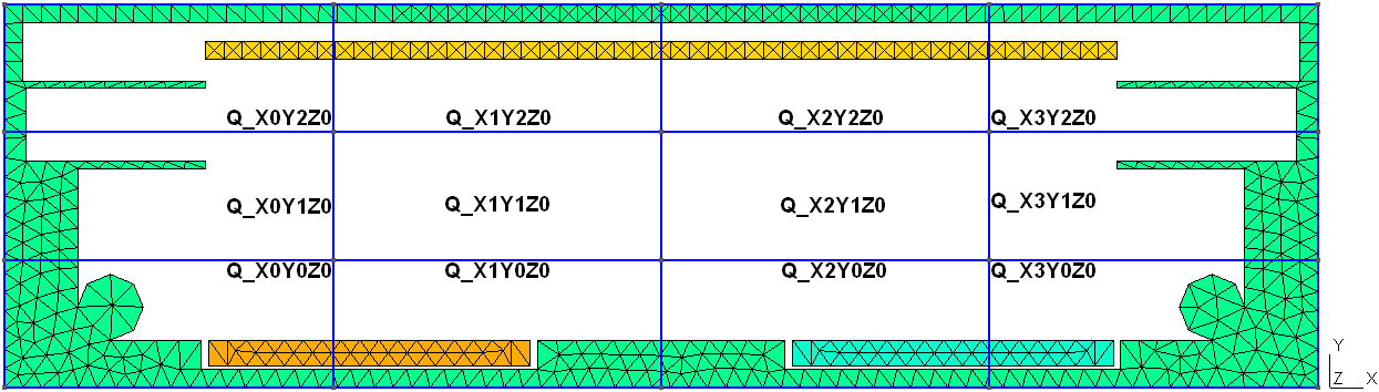
All particles entering or leaving the quad are multiplicated/deleted depending on the nreal factor quotient of the involved quads.
2.1.15 User actions and functions
block User_Block: {
};
The User_Block is executed once before the time cycles start and can be used for combining DMSC and PIC-MC simulations (time scale splitting) as shown in this example
block User_Functions: {
};
In the User_Functions block it is possible to include user defined functions for use during the simulation, more information can be found in following section.
2.1.16 User functions
In this block it is possible to include user defined functions for use during the simulation, e.g. a special voltage function. The syntax is the following:
type function_name(variable_name=type) = {
  return calculated_value;
};
The type of the function as well as the variables can be "integer" or "float", the names of both are arbitrary but have to start with a letter. The number of variables is not limited and the calculated value can include common mathematical functions. An example of such a user function is the modulo function:
float myModulo(dividend=float, divisor=float) = {
  integer quotient = dividend / divisor;
  return dividend - quotient * divisor;
};
The use of this user function in the voltage function of an electrode would be e.g.:
vf = "-VP*myModulo(TIME, PAR.PERIOD)+DC_BIAS";2.1.17 Species and cross sections
SPECIESFILE = "my_species_definition.r";
SIGMAFILE   = "my_sigma.r";
If you want to use alternative or additional species not included by default, you have to specify the name of your own file in SPECIESFILE. Normally you then also have to specify your own SIGMAFILE which includes the cross sections of the new species. The list of all available species can be found in section (sec:prep_species_list?).
SIGMA_DEBUG  = 1;
SIGMA_ENERGY = 2000.0;
By activating SIGMA_DEBUG (setting the value to 1) one text file for each collision cross section in use is written to the simulation folder. This data can be beneficial if you want to show the curves in a presentation. The SIGMA_ENERGY parameter can be used to manually set the limit in eV up to which the cross sections are calculated. Since the default value is 1100.0 eV, you may get some warning messages if you have strong electric fields and particle energies are higher than the limit.
2.1.18 Debugging
DEBUG       = 0;
NTESTCYCLES = 200;
The DEBUG mode is switched off (= 0) by default, but can be switched on (= 1) if your simulation does not start properly and you want to know exactly what's the problem. The output can be quite long, so consider redirecting it to a file.
The default number of test cycles for the load measurement ahead of every simulation shutdown is 200, which should be appropriate for the most cases. Changing this can be done by setting NTESTCYCLES to the desired value. Depending on these measurements a load balancing is carried out, if you restart a simulation and the number of quads is higher than the number of requested CPUs.