DSMC and PICMC documentation

1.1 Collision routine

In order to treat the collision dynamics in proper resolution, the simulation volume is divided into simulation cells, whereof the cell spacing \(\delta x\) is less than the mean free path \(\lambda\). In these cells, the collision is treated with a statistical approach, which is called no time counter (NTC) - method. This method rather estimates the number of collisions in a simulation cell per time step instead of checking all possible particle trajectory intersections. The latter is quite time consuming and would scale with the square of the particle number.

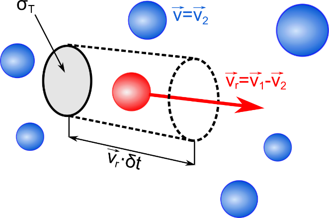
The estimation on the number of collisions is based on a model shown in Figure 1.1. Let us assume we have a particle class, whereof each particle has a velocity \(v_2\) and let’s assume an inertial system, where \(v_2=0\). For a test particle with velocity \(v_1\), its cross section \(\sigma_T\) for collisions with particles of the class \(v_2\) can be considered as a circular area. If we multiply this area with the test particle’s trajectory during time step \(\delta t\), a cylindrical volume results. This volume is now put in ratio with the cell volume \(V_c\), which yields the collision probability

\[p_{12} = \frac{\sigma_T v_r \delta t}{V_c}\](1.1)

Here, \(v_r = |\vec{v}_1-\vec{v_2}|\) is the relative velocity between two potential collision partners, and \(\sigma_T\) is their total cross section. Equation (1.1) says that the collision probability basically is proportional to the product \(\sigma_T v_r\). In general, \(\sigma_T\) depends on the relative velocity and other parameters. For a good initial estimate of the expected number of collisions, it is useful to take the maximum possible product of cross section and relative velocity, \(<\sigma_T v_r>_{max}\), which can be obtained from the energy-dependent cross section curve. Based on this, the maximum possible collision probability is

\[p_{12.max} = \frac{<\sigma_T v_r>_{max} \delta t}{V_c}\](1.2)

For two particle species 1, 2 with particle numbers of \(N_1, N_2\) per cell and a statistical weight factor of \(N_R\), the maximal expected number of collisions becomes

\[N_{\textrm{preselect}} = \frac{N_R N_1 N_R N_2}{N_R} p_{12.max} = N_R N_1 N_2 p_{12.max}\](1.3)

In the NTC method, a number of \(N_{\textrm{preselect}}\) pairs of collision partners is randomly selected from the particles within a cell. For each pair, their actual value of the product \(\sigma_T v_r\) divided by \(<\sigma_T v_r>_{max}\) is their relative collision probability. Based on that, the collision takes place with the selected particles, if the following random experiment succeeds:

\[r\# < \frac{\sigma_T v_r}{<\sigma_T v_r>_{max}} \](1.4)

Here, \(r\#\) is a random number between 0 and 1. The situation gets a bit more complicated in case of two collision species 1,2 and a reaction product 3 with different statistical weights \(N_{R1}, N_{R2}, N_{R3}\). In this case, the number of pre-selected collision pairs is computed via

\[N_{\textrm{preselect}} = \frac{N_{R1} N_1 N_{R2} N_2}{\min(N_{R1}, N_{R2}, N_{R3})}\times p_{12.max}\](1.5)

Note that now, the collision partner or reaction product with the least statistical weight is determining the number of to be preselected collision pairs. The decision, whether a collision for a randomly chosen pair actually takes place is again made via Equation (1.4). After the collision it still has to be considered that the collision partners and reaction products all have different weight factors. Therefore, for each species \(i\) a post-collision probability \(w_i\) decides, whether the collision actually takes effect or not:

\[w_i = \frac{\min(N_{R1}, N_{R2}, N_{R3})}{N_{Ri}}\](1.6)

Example: Let Ar have a statistical weight of \(N_{R.Ar} = 10^{10}\) and electrons and ions each have \(N_{R.e}, N_{R.i} = 10^5\). After an ionization collision

\[\textrm{Ar}+e^- \rightarrow \textrm{Ar}^+ + 2e^-\](1.7)

equation (1.6) yields post-collision probabilities for electrons and ions of 1.0 and for Argon \(w_{Ar} = 10^{-5}\). Thus, in each performed ionization collision, an electron and ion is actually created but the Ar neutral with the much heigher statistical weight is deleted in only 1 out of 100000 cases. The same principle holds for the modification of the collision partner’s velocities.

There is the additional complication that some of the species might be frozen. In this case, equation (1.5) is modified as follows.

\[N_{\textrm{preselect}} = \frac{N_{R1} N_1 N_{R2} N_2}{\min(\textrm{statistical weights of all non-frozen species})}\times p_{12.max}\](1.8)

The post-collision probability is analogously modified to

\[w_i = \frac{\min(\textrm{statistical weights of all non-frozen species})}{N_{Ri}}\](1.9)

In case of frozen species they do not exist in form of particles but merely with time-averaged values for the particle density \(<n>\), their cartesian velocity components \(<v_x>, <v_y>, <v_z>\) and their square velocity \(<v^2>\). From these values, test particles for the collision can be generated. First, their kinetic temperature \(T\) can be computed from the velocity averages by

\[T = \frac{m}{3k_B}\left\{<v^2>-<v>^2\right\},\,\textrm{with }<v>=\sqrt{<v_x>^2+<v_y>^2+<v_z>^2}\](1.10)

Here, \(m\) is the atomic mass of the frozen species, and \(k_B\) is the Boltzmann constant. From the temperature and mass, velocity components can be randomly chosen according to the following method

\[v = \sqrt{-\frac{2k_B T \ln(r\#)}{m}}, \phi=2\pi r\#, v_1=v\sin(\phi), v_2=v\cos(\phi)\](1.11)

Unfortunately, equation (1.11) yields only two velocity components \(v_1, v_2\) while a real particle needs three. Thus, (1.11) is executed two times, and three velocity are selected out of the four.