
DSMC and PICMC documentation
2022-02-17
4.1 Cylindrical tube flow - optimized domain decomposition
While the concept of embedding the whole mesh geometry into a single "bounding box" is simple and user-friendly, this method is not always efficient. In some cases, only a small fraction of the simulation volume will be actually used; thus the simulation model will consists of a majority of empty cells. In other cases, there may be big pressure differences within the simulation volume, which makes the definition of strongly varying cell dimensions necessary. With one single bounding box, this is not always possible in a flexible manner.
For this purpose, it is possible since picmc version 2.3.4 to use multiple joined rectangular bounding boxes as simulation volume:
- The bounding boxes can be defined in the parameter file with ''block MQUAD: { ... }; ''
- The connections between the bounding boxes are defined within ''block MJOIN: { ... }; ''
- If these blocks are omitted (or commented out), picmc will use the previous method of a large single bounding box.
- Due to limitations of the electric field solver with respect to multi-gridding schemes, the MQUAD / MJOIN feature is currently only available for DSMC simulation (WORKMODE=0 in the parameter file).
An example of the usage of multiple bounding boxes is shown in the following picture; it is based on the same tube geometry as in the DSMC example of section (sec:dsmc_example_1?).
| Single box with wasted simulation volume | Use of multiple boxes |
|---|---|
 |
 |
In the following, it will be shown how to realize the multiple boxes arrangement in the parameter file.
4.1.1 Tube example with four bounding boxes
In the tube example of the previous section, we have an inlet and an outlet chamber which are connected by a long tube. With one single bounding box, the simulation volume has a much larger cross section than the tube diameter resulting in a large number of wasted simulation cells. Thus, we would like to divide the simulation volume into the following bounding boxes,
- one for the inlet region,
- one for the left side of the tube with higher pressure,
- one for the right side of the tube with lower pressure,
- one for the outlet region.
The GEO and PAR file of the tube example with multiquad approach can be downloaded here as ZIP file.
4.1.1.1 Definition of multiple bounding boxes in block MQUAD
In order to define that in the parameter file, a block MQUAD must be defined. Within this block, all desired bounding boxes have to be defined as shown in the following:
# ... geometry definition within parameter file

UNIT = 0.001; # Unit of mesh geometry

block MQUAD: {

  block Left: {
    DIV_X = [23, 23, 23, 23, 23]; NX = [4, 4, 4, 4, 4];
    DIV_Y = [140, 140, 140];      NY = [28, 28, 28];
    DIV_Z = [140, 140, 140];      NZ = [28, 28, 28];
    X0 = -110; Y0 = -210; Z0 = -210;
    NREAL_SCALE=0.5;
  };

  block Tube1: {
    DIV_X = [65, 65, 65]; NX = [12, 10, 8];
    DIV_Y = [105];        NY = [20];
    DIV_Z = [105];        NZ = [20];
    NREAL_SCALE_X = [0.5, 0.5, 1];
  };

  block Tube2: {
    DIV_X = [195]; NX = [18];
    DIV_Y = [105]; NY = [10];
    DIV_Z = [105]; NZ = [10];
  };

  block Right: {
    NX=[12]; DIV_X=[115];
    NY=[8, 8, 8]; DIV_Y=[140, 140, 140];
    NZ=[8, 8, 8]; DIV_Z=[140, 140, 140];
  };
};
The following information is to be specified:
For each bounding box, a block has to be specified with the following syntax:
block boundingbox_name: {
# ... all parameters of the
# ... bounding box go here
};
The geometric dimension in X, Y, Z direction is specified in the arrays DIV_X, DIV_Y, DIV_Z. If e. g. a box extends over 195 mm in X direction and should have three segments whereof each extends 65 mm, the specification reads:
DIV_X = [65, 65, 65];If only one segment in X direction is needed, the line reads:
DIV_X = [195];The number of cells for each sub-segment in X, Y and Z direction is specified in the arrays NX, NY, NZ. The number of entries in e. g. NX must be the same as the number of entries in DIV_X.
Further, it is now possible to specify a different NREAL particle weighting factor in each bounding box. This is performed by specifying:
NREAL_SCALE = 0.5;which means, that the particle weighting factor within this bounding is 50% of the global particle weighting factor.
In case of a sub-segmentation It is also possible to specify different weighting factors for each segment along one of the directions X, Y, Z. If we have e. g. three sub-segments along X direction it is possible to specify three different weighting factors by:
NREAL_SCALE_X = [0.25, 0.5, 1];Exactly one of the bounding boxes needs absolute coordinates, these are to be specifed in the variables X0, Y0, Z0. The line:
X0 = -110; Y0 = -210; Z0 = -210;means, that the lower coordinate edge of the bounding box is located at (-110, -210, -210). The unit of the coordinates is given in the UNIT variable in the parameter file. The absolute coordinates of the other bounding boxes will be automatically determined, when all boxes are joined together (see below).
4.1.1.2 Joining multiple bounding boxes together in block MJOIN
After specifying the dimension, segmentation and cell numbers of all bounding boxes, they have to be joined together in order to form a contiguous simulation volume. For this purpose, the block MJOIN is used in the parameter file as shown in the following lines.
block MJOIN: {
  Left.join(Tube1,  "x", -160, -160);
  Tube1.join(Tube2, "x",    0,    0);
  Tube2.join(Right, "x",  160,  160);
};
As can be seen, adjacent boxes are connected via the join command, whereof the syntax is box1.join(box2, "side", da, db);. The meaning of the parameters is as follows:
box1, box2= The names of the boxes which are to be joined.side= The direction of the junction, can be either"x","y"or"z".da, db= If the junction areas of both boxes are different, a coordinate offset is needed to specify the lateral coordinate offset between both boxes.
For the offsets, the coordinates a and b are the remaining axes which are vertical to the junction direction. The offsets are obtained by drawing a vector from the lower edge of the second box to the lower edge of the first box. Example: If the coordinates of the lower edges are (x1, y1, z1) for the first box and (x2, y2, z2) for the second box, we can obtain the offsets according to Table 4.2.
| Join direction | Direction of a | Direction of b | Offset da | Offset db |
|---|---|---|---|---|
| x | y | z | y1-y2 | z1-z2 |
| y | x | z | x1-x2 | z1-z2 |
| z | x | y | x1-x2 | y1-y2 |
Generally, if the lower edge of the second box is positioned within the surface of the first box, the offset is negative. Otherwise it is positive. Examples are given in the following figure:
| Second box fits within first box surface | First box fits within second box surface |
|---|---|
 |
 |
In case if all boxes are joined central-symmetrically, there is no need to calculate the offsets manually. Instead, the command box1.join_center(box2, "side"); can be used, where the offset parameters are omitted. Our tube example has central-symmetric junctions; thus, the MJOIN block can be simplified to
block MJOIN: {
  Left.join_center(Tube1,  "x");
  Tube1.join_center(Tube2, "x");
  Tube2.join_center(Right, "x");
};
4.1.1.3 Former join_rect function
In picmc versions prior 2.4.0.5 only the join_rect function was available within the block MJOIN. For backwards compatibility reasons, this function can still be used; however, for new simulation cases it is recommended to use the join command instead.
With the join_rect command, our MJOIN block would look like follows:
block MJOIN: {
  Tube1.join_rect(Tube2, "x", 0, 0, 105, 105,     0, 0);
  Tube2.join_rect(Right, "x", 0, 0, 105, 105,     160, 160);
  Left.join_rect(Tube1,  "x", 160, 160, 260, 260, 0, 0);
};
Generally, the syntax of the join_rect command between two boxes - "FirstBox" and "SecondBox" - is as follows:
FirstBox.join_rect(SecondBox, "direction", a0, b0, a1, b1, delta_a, delta_b);with the following parameters:
FirstBox,SecondBox= The names of the bounding boxes as defined in blockMQUAD. The box with the lower coordinates (with respect to the direction of the junction) should always be specified first asFirstBox, the other box with higher coordinates will be theSecondBox.- For
"direction"chose either"x", "y", "z". This is the direction of the junction. - The parameters a0,b0,a1,b1 specify the position of the rectangular orifice in relative coordinates with respect to the first box.
- The parameters delta_a, delta_b specify the offset of the rectangular orifice in relative coordinates with respect to the second box.
4.1.1.4 Examples of the join_rect function
The usage of the join_rect command is demonstrated on two examples. In the first example, a big bounding box is joined to a smaller bounding box along X direction:
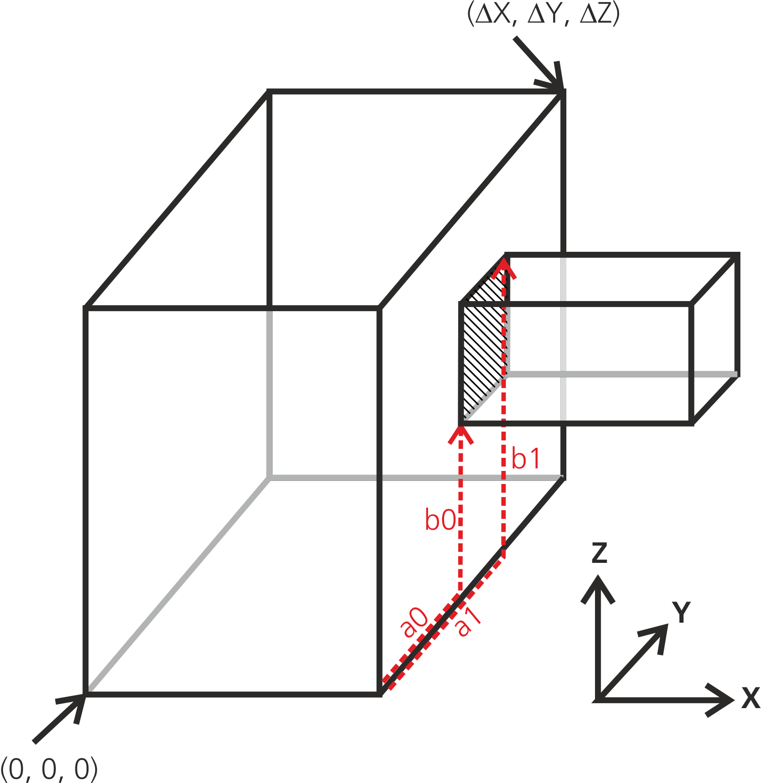
Here, the first box is joined to the second box via the hatched rectangular area. Since the hatched area is smaller than the full right side of the first box, the position of the rectangular area within the right side can be freely chosen. It spans between the coordinates (a0, b0)-->(a1, b1). In the given coordinate system, the connection is performed along X direction; then the a coordinate is parallel to Y, and the b coordinate is parallel to Z. The coordinate conventions are shown in the table in the previous section.
It has to be mentioned again, that the (a0, b0)-->(a1, b1) coordinates are relative with respect to the first box, i. e.
\(0 \le a0, a1 \le \Delta Y\textrm{ and }0 \le b0, b1 \le \Delta Z\)
Since the hatched junction surface is identical with the left surface of the smaller right box, the offset (delta_a, delta_b) is (0, 0) in this case.
The opposite situation occurs, if a smaller bounding box is joined to a bigger one:
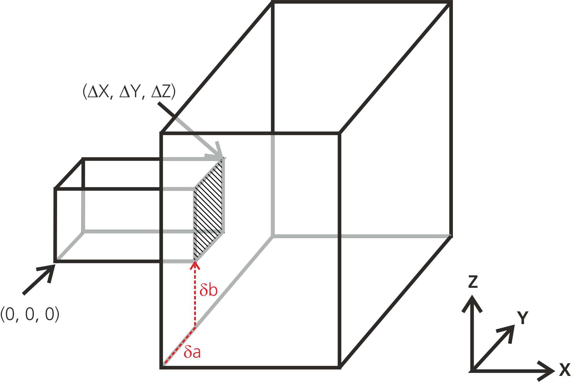
Here, the hatched junction surface completely fills out the right surface of the first bounding box. Thus, the surface coordinates are
\((a0, b0) = (0,0)\)
\((a1, b1) = (\Delta Y, \Delta Z)\).
Now, the position of the junction surface within the left surface of the second box can be freely adjusted via the offset coordinates (delta_a, delta_b). Thus, the full command would read like
FirstBox.join_rect(SecondBox, "x", 0, 0, Delta_X, Delta_Y, delta_a, delta_b);