1 Introduction to the DSMC / PIC-MC software package

1.1 The Direct Simulation Monte Carlo (DSMC) - and Particle-in-Cell Monte-Carlo (PIC-MC) methods

The simulation of transport phenomena is an important method to understand the dynamics in low-pressure deposition reactors. This includes the flow of the process gas as well as the transport of reactive gases and precursors. The most general transport equation in classical mechanics is the Boltzmann transort equation

\[\left(\frac{\partial}{\partial t}+\vec{v}\nabla_{\vec{x}}+\frac{\vec{F}}{m}\nabla_{\vec{v}}\right) f\left(\vec{x}, \vec{v}, t\right) = \left.\frac{\partial f}{\partial t}\right|_{collision}\](1.1)

It describes the time evolution of a particle distribution function \(f\left(\vec{x}, \vec{v}, t\right)\) in a 6-dimensional phase space (space and velocity). Such high-dimensional spaces are usually difficult to handle by numerical simulation, e.g. by the finite element method, because the number of mesh elements would increase with the 6^th power of the geometric scale. A pertubation analysis (see e.g. Chapman and Cowling (1970)) shows that for a low value of the mean free path (see section (sec:num_constraints_dsmc?)) in comparison to characteristic geometric dimensions of the flow, the Boltzmann equation can be approximated by the Navier Stokes equations, which merely treat the density, velocity and pressure as flow variables in the three-dimensional space. For the Navier Stokes equations, a large variety of solvers based on Finite Element or Finite Volume Method (FEM, FVM) are available as commercial or open-source codes. A prominent FVM based solver for continuum mechanics is OpenFOAM, whereof different versions are maintained either by the OpenFOAM Foundation or by the ESI Group. Both version differ slightly with respect to the included solvers and auxiliary libraries.

The validity of the Navier Stokes equations depends on the mean free path \(\lambda\) with respect to characteristic geometric dimensions \(d\), which can be expressed as the so-called Knudsen number

\[Kn = \frac{\lambda}{d}\](1.2)

As shown in Figure 1.1, continuum approaches are only valid for Knudsen numbers well below 0.1. For higher Knudsen values, kinetic simulation codes must be used instead. In case of very large Knudsen numbers \(Kn>>1\), the flow can be considered as collisionless; in this case it is possible to use a ray-tracing approach for solving the Boltzmann equation via a particle based approach. An example of a software which solves particle transport under molecular flow conditions is MolFlow developed at CERN. A more detailed discussion on thin film deposition methods and simulation codes is given in Pflug et al. (2016).

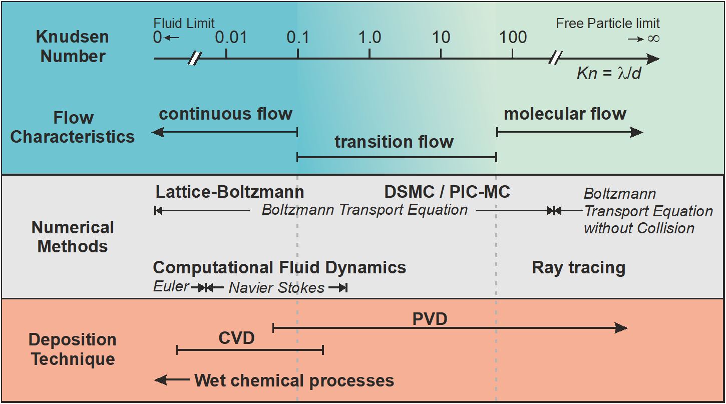
For an intermediate range \(0.1<Kn<100\) of the Knudsen number, neither a continuum approach nor a solver based on collisionless flow is viable. With respect to thin film deposition technology, most Physical Vapor Deposition (PVD) and some of the Chemical Vapor Deposition (CVD) processes fall into this intermediate range with respect to their process conditions. Thus, their proper modeling requires to use a kinetic solver of the Boltzmann equation including collision term.

Other than a fully-fledged FEM or FVM based solution of the Boltzmann equation, a statistical approach called Direct Simulation Monte Carlo (DSMC) - method (see Bird (1994)) is a solution method with feasible computational effort. It is based on following simplifications:

• All flow species are represented by super particles, a super particle has the same mass and properties as real gas molecules of the respective species but represents a number \(N_{R.species}\) or NREAL_SPECIES of real particles. The scaling factor is necessary as otherwise the number of particles to be simulated would be too high to fit into usual high performance computing hardware.
• For collisions between particles, only binary collisions are considered.
• For performance reasons, the particle movement and collision are treated not simultaneously but in two separate routines, which are invoked subsequently for each time cycle.

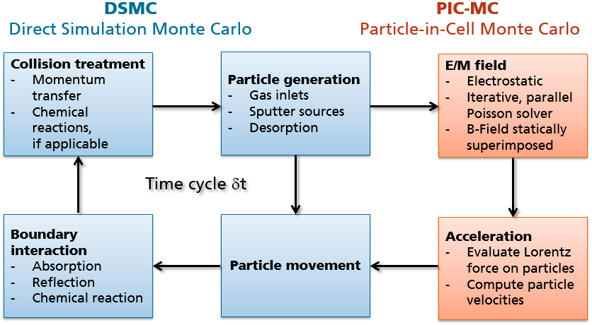
The 3^rd simplification requires that the product \(\delta t \times \overline{v}\) of time step and mean thermal velocity \(\overline{v}\) of all treated species is below the cell spacing of the simulation grid. A typical schedule of the time step in a DSMC solver can be seen in Figure 1.2 by following the blue boxes.

The DSMC method only treats the transport of neutral particles and hence is suitable to model rarefied gas flows, evaporation or thermal CVD processes. If the transport of charged particles becomes relevant as in plasma processes, the electric and magnetic fields have to be additionally considered. The approximation used in this software is referred to as Vlasov Poisson equation, which means that the force term in Equation (1.1) is replaced by the Lorentz force,

\[\left(\frac{\partial}{\partial t}+\vec{v}\nabla_{\vec{x}} +\frac{q}{m}\left\{\vec{E}+\vec{v}\times\vec{B}\right\}\nabla_{\vec{v}}\right) f\left(\vec{x}, \vec{v}, t\right) = \left.\frac{\partial f}{\partial t}\right|_{collision}\](1.3)

and the electric potential \(\phi\) is derived from the Poisson equation according to the actual charge density distribution \(\rho\) and the relative dielectric permeability \(\epsilon_r\) of the background.

\[\Delta\phi + \frac{\nabla\epsilon_r\nabla\phi}{\epsilon_r}= -\frac{\rho}{\epsilon_0\epsilon_r}\](1.4)

In a self-consistent Particle-in-Cell Monte Carlo (PIC-MC) - simulation, equations (1.3) and (1.4) have to be fulfilled simultaneously, while in the actual iterative implementation they are solved sequentially - as shown by the large cycle in Figure 1.2. This imposes additional numerical constraints on the simulation parameters such as cell spacing, time step etc. as elaborated further in section (sec:num_constraints_picmc?). A detailed discussion of the PIC-MC method is given in the monography of Birdsall and Langdon (2005).

1.2 PICMC installation instructions

1.2.1 Installation of the software package

The DSMC / PICMC package is usually being shipped as compressed tar archive, such as picmc_versionNumber.tar.bz2. In order to uncompress it, the following command can be used:

 tar xjvf picmc_versionNumber.tar.bz2

This will create an installation folder picmc_versionNumber/* where the required binaries, libraries and script files are included. The meaning of the sub folders are as follows:

• picmc_versionNumber/bin = the C++ compiled binaries including picmc worker task, magnetic field computation module bem and the script interpreter rvm.

• picmc_versionNumber/lib = compiled run time libraries used by the script interpreter rvm.

• picmc_versionNumber/scr = scripts used by rvm for scheduling the simulation run and managing the input and output data as well as internal model parameters (including species and cross sections)

• picmc_versionNumber/sh = Linux shell scripts (bash) for submitting simulation runs

• picmc_versionNumber/data = Tabulated cross section data for some species

After creation of the installation folder picmc_versionNumber/ it shall be moved into an appropriate installation directory, e.g.

mv picmc_versionNumber /opt/picmc

In the home directories of the users, appropriate environment variable settings need to be included into their /home/user/.bashrc files. A possible way is to include the following lines:

export PICMCPATH=/opt/picmc/picmc_versionNumber
export LD_LIBRARY_PATH=$PICMCPATH/lib:$LD_LIBRARY_PATH
export RVMPATH=$PICMCPATH/rvmlib
export PATH=$PICMCPATH/bin:$PICMCPATH/sh:$PATH

The part after PICMCPATH= has to be replaced by the path of your actual installation directory. After changing the .bashrc the users are required to close their command prompt and open a new one in order for the changes to take effect.

The direct invocation of simulation runs is done via the script picmc_versionNumber/sh/rvmmpi. In order for this to work correctly, the correct path of your OpenMPI installation directory has to be specified in this file. The respective line can be found in the upper part of the file and shall look like follows:

MPI_PATH=/opt/openmpi-2.1.0

Please replace this path with the correct installation directory of OpenMPI for your Linux machine.

1.2.2 Job submission via the SLURM job scheduler

In case of the SLURM job scheduler, we provide a sample submission script which is given here in submit.zip. Unpack this ZIP archive and place the script submit into an appropriate folder for executable scripts such as /home/user/bin or /usr/local/bin. Don't forget to make this script executable via chmod +x submit.

In the upper part of the script, there is an editable section which has to be adjusted to your actual SLURM installation:

# ======================
# Editable value section
# ======================

picmcpath=$PICMCPATH                  # PICMC installation path
partition="v3"                        # Default partition
memory=1300                           # Default memory in MB per CPU
walltime="336:00:00"                  # Default job duration in hhh:mm:ss 
                                      # (336 hours -> 14 days),
                                      # specify -time <nn> of command line 
                                      # for different job duration
MPIEXEC=mpiexec                       # Name of mpiexec executable
MPIPATH=/opt/openmpi-2.1.0            # Full path to OpenMPI installation
#MAILRECIPIENT=user@institution.com   # Switch to get status emails from SLURM
                                      # (Requires a functional mail server)

QSUB=sbatch

# =============================
# End of editable value section
# =============================

It is important to specify the correct OpenMPI installation path in MPIPATH as well as the default SLURM partition under partition. Additionally, the approximate maximal memory usage per task and maximal run time of the job are to be specified in memory and walltime. In the settings shown above, there is a maximal memory allocation of 1.3 GB per task and a maximal run time of 14 days. These settings can be overwritten by command line switches of the submit script. The submit script can be invoked in the following ways:

All above examples assume that your simulation case is given in the file simcase.par in the actual directory. By submitting a SLURM job via submit the following additional files will be created:

• simcase-out.txt: The screen output in stdout; this file is being refreshed typically every 15-30 seconds.

• simcase-err.txt: Error messages (if any) can be found here. If the simulation crashes or behaves in an unexpected way, it is important to look into this file.

• simcase.slurm: This is a native SLURM submission script generated by submit according to the actual settings as specified in the command line. If the job needs being re-submitted with the same settings, it can be easily done via sbatch simcase.slurm

1.3 General workflow

For DSMC-Gasflow simulation, PIC-MC plasma simulation or BEM magnetic field computation, different work flows are required. Depending on the usage of a Grid Scheduler or direct call of mpirun, the invocation commands may differ. In the following, the work flows and invocation commands for the different simulation cases are summarized.

1.3.1 DSMC gas flow simulation

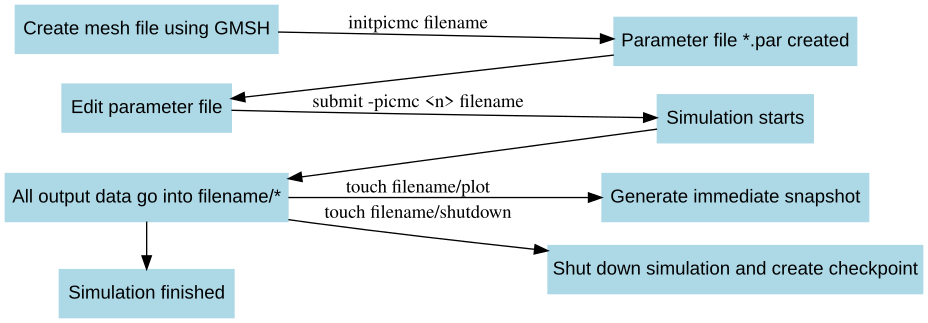
The work flow in a DSMC gas flow simulation can be summarized as follows:

1. Create geometric mesh file of the simulation domain (e. g. filename.msh) via GMSH and save mesh file e. g. as filename.msh

2. Create parameter template filename.par out of mesh file filename.msh

   • initpicmc filename

3. Edit the parameter file filename.par with an ASCII editor of your choice.

4. Start DSMC simulation

   • Via mpirun direct call: rvmmpi [-hostfile <hostfile>] -picmc <n> filename

   • Via SLURM submit script: submit -picmc <n> filename

5. Create intermediate snapshots during simulation immediately

   • touch filename/plot

6. Shutdown simulation and create simulation checkpoint (for the purpose of later continuation)

   • touch filename/shutdown

7. Kill a simulation immediately without writing a checkpoint

   • touch filename/kill

8. Restart a simulation run from last checkpoint

   • Same command as in step 4.

The number of parallel picmc tasks, which should be used during computation are given in the <n> parameter after the -picmc switch. Remember that the number of parallel picmc tasks may not exceed (but may be less than) the number of segments of the simulation domain. The actual number of allocated CPU cores will be one more than the number of picmc tasks, since one more task is required for the master process.

If the simulation is invoked directly via mpirun using the rvmmpi script, a hostfile must be declared. This hostfile contains the names of the computing nodes together with their available number of CPU slots. An example is given in the following:

node1 slots=1
node3 slots=48
node4 slots=48

If a batch scheduler such as LSF or Sun Grid Engine (SGE) is used, no hostfile must be specified since the hostfile will be created dynamically by the scheduler. A graphical visualization of the work flow is given in Fig. 1.3.

1.3.2 PIC-MC plasma simulation without magnetic field

For a PIC-MC plasma simulation without magnetic field (e. g. in a PECVD parallel plate reactor or a glow discharge without magnetic field), the workflow is the same as in the DSMC case.

1.3.3 PIC-MC plasma simulation with magnetic field

For a plasma simulation with an overlying magnetic field - e. g. a discharge of a magnetron sputtering target - additional steps for producing the magnetic field are required prior to starting the picmc simulation. The complete workflow is summarized in the following:

1. Create geometric mesh file of the simulation domain (e. g. filename.msh) via GMSH and save mesh file e. g. as filename.msh

2. Create geometric mesh file of the magnetic arrangement (e. g. magnet.msh) via GMSH and save mesh file e. g. as magnet.msh

3. Create parameter template filename.par out of mesh file filename.msh

   • initpicmc filename

4. Edit the parameter file filename.par, and insert the name of the magnetic mesh file in the field BEMMESH.

5. Create a template file filename.bem, where the domain numbers and surface polarizations of the magnets are specified.

   • initbfield filename

6. Edit the magnetic template file filename.bem

7. Perform magnetic field computation

   • Via mpirun direct call: rvmmpi [-hostfile <hostfile>] -bem <n> filename

   • Via SLURM submit script: submit -bem <n> filename

8. Start PIC-MC simulation

   • Via mpirun direct call: rvmmpi [-hostfile <hostfile>] -picmc <n> filename

   • Via SLURM submit script: submit -picmc <n> filename

9. Create intermediate snapshots during simulation immediately

   • touch filename/plot

10. Shutdown simulation and create simulation checkpoint (for the purpose of later continuation)

    • touch filename/shutdown

11. Kill a simulation immediately without writing a checkpoint

    • touch filename/kill

12. Restart a simulation run from last checkpoint

    • Same command as in step 8.

References