From plasma to a coated lens
PICMC does not simulate a coating process on its own. It is one stage in a chain of simulation codes that starts with the geometry of a coater and ends with a predicted or explained coating result: layer thickness on a curved substrate, an optimised mask, the energy distribution of the particles that arrive at the surface. This page shows that chain and what comes out of it, so the single-stage documentation is easier to place.
The rest of this documentation describes PICMC itself. Here the question is the opposite one: which part of a coating problem does PICMC answer, what does it hand to the next stage, and what does it need from the stage before.
Why a chain instead of one code
Each stage of a sputter process lives on its own length and time scale, and each one needs a different numerical method. A plasma needs the motion of individual electrons and ions; the transport of sputtered atoms through metres of chamber is a molecular flow problem; the film that grows on the substrate is a surface process on the scale of nanometres.
- Make the invisible visible. The ion and neutral flux that hits the target and the substrate is what determines the result, and it cannot be measured inside a running coater. Simulation gives access to it.
- Virtual prototyping. Chamber, shields, masks, targets and substrate motion can be varied before hardware is touched — including geometries that do not exist yet.
- Pre-optimisation of large lines. An industrial coater can be designed in-silico long before it is built.
- Fewer trial runs. A well-designed parameter study replaces a series of coating runs, which saves time, cost and material.
The chain
The picture below is the pipeline as it is used for optical coatings: first the plasma and the sputter source, then the way back to the substrate.
Read it as two halves. The upper half answers "how much material leaves the target, and where"; the lower half answers "where does it land, and how do I shape the flux so that it lands evenly". PICMC owns the first half up to the erosion profile.
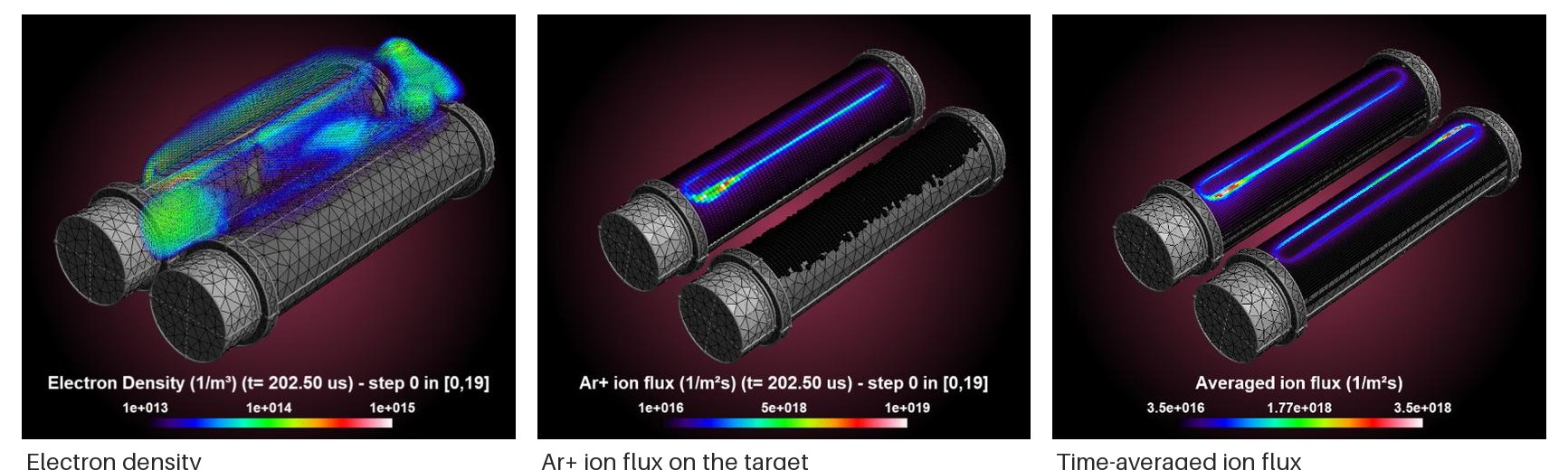
The PICMC stage for a source with two cylindrical targets: electron density, Ar⁺ ion flux on the target, and the time-averaged flux from which the erosion profile is derived. Source: Pflug, A. et al., Proc. 15th ISSP (2019).
The chain is meant to be run in a loop
The two dashed arrows are the actual point of the framework. A single pass through the chain gives one prediction; a digital twin is what you get when the pass is repeated with changed inputs, and the interesting part is deciding which inputs to change:
- Inner loop, mask and geometry. The source stays as it is, only the mask, the shielding or the substrate motion is adapted until the thickness profile on the part matches the target. This loop is cheap because the plasma stage does not have to be repeated, and it is the loop that is automated today (see the release notes for release 26 below).
- Outer loop, everything upstream. If the target cannot be reached by shaping the flux, the cause is on the source side: target geometry and erosion, gas pressure and composition, magnetic field, shields, or the material of the target itself. Then the plasma stage is re-run with changed parameters, and the inner loop starts again.
Doing this by hand is a parameter study. Doing it automatically needs a goal function — a rate profile, a spectrum, a uniformity number — and a simulation that is fast and stable enough to be called a few dozen times. Both are what the framework is built for.
Stage by stage
| Stage | Done by | Needs | Delivers |
|---|---|---|---|
| Background gas and magnetic field | DSMC, field computation | Geometry, pressures, gas composition, target currents | Gas density and flux field, magnetic field for the plasma stage |
| Plasma | PICMC | Geometry, gas field, magnetic field, species and cross-sections | Electron and ion density, potential, ion flux on every surface |
| Erosion profile | PICMC (time-averaged ion flux) and the sputter yield | Ion flux, target material, impact angles | Erosion depth along the racetrack |
| Sputter transport | DSMC | Erosion profile, gas background | Flux of sputtered atoms towards the substrate, angular and energy resolved |
| Deposition on the substrate | Ray tracing | Atom flux, substrate motion, mask geometry | Local deposition rate on the real part |
| Mask and geometry | Optimisation loop around the two stages above | A goal function, e.g. a rate profile that compensates the substrate curvature | Mask shape, substrate motion, shielding |
| Verification | Measurement | Coated part | Spectra, thickness profiles, particle contamination |
Every stage can also be used on its own. Most questions do not need the whole chain — a plasma question often ends at the ion flux, a uniformity question starts with a measured or estimated erosion profile.
What PICMC contributes to the chain
- Ion flux on surfaces. Time-averaged fluxes are written as cell-centred fields and are the input for the erosion estimate. Without the averaging over many RF periods the flux is too noisy to integrate.
- Angular and energy distributions. Particles that cross a boundary — a membrane, a monitor substrate — can be recorded as histograms of impact angle and energy. Downstream atomistic growth simulations need exactly that, not a single mean value.
- Collision and surface statistics. Where particles collide, where they are absorbed or desorb, how much energy a surface receives: this is what explains a profile rather than just predicting it.
- Restartable long runs. A plasma stage for a real coater geometry runs for hours to days; checkpoints make it possible to stop after the plasma has settled and continue with a changed downstream setting.
Examples
In-line hot-wire CVD coater
A DSMC model of an in-line HWCVD coater in two and three dimensions produces the silicon thickness profile on the moving carrier. The computed profile was compared with the interference colour of the coated steel carrier — a cheap and very sensitive check of the whole transport model, because a few percent of rate difference changes the colour.
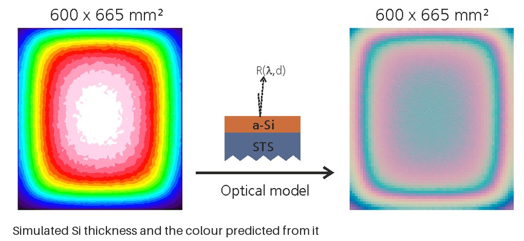
Simulated Si thickness on the 600 × 665 mm² carrier and the interference colour computed from it with an optical model.
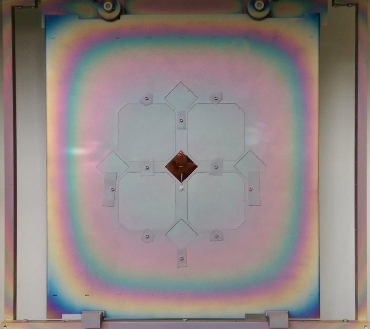
The coated steel carrier: the interference colour is the check.
Reactive sputtering of TiO₂ with atomistic growth
A coupled DSMC / PIC-MC simulation of reactive TiO₂ sputtering including ionised species and negative O⁻ ions, followed by a kinetic Monte Carlo growth simulation. Samples perpendicular and tilted at 70° in the centre and off-centre position. The model reproduces the difference between metallic, oxide and transition mode — the regime where the process is hardest to keep stable.
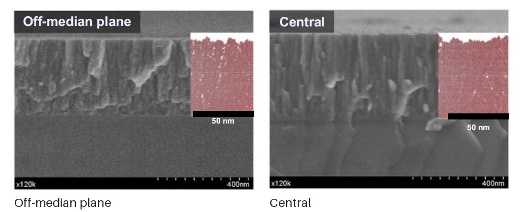
Cross-sections of the grown TiO₂ film, each perpendicular and tilted by 70°, at off-median position and in the centre, with a segmented inset for the column analysis. Source: Tonneau, R. et al., J. Phys. D: Appl. Phys. 54 (2021) 155203.
Bandpass filter on a convex lens
The problem: a bandpass filter deposited on a convex lens shifts towards shorter wavelengths at the edge, because the deposition rate drops with curvature and the angle of incidence grows. At the edge the effective thickness is about 95 % at 16°, and the passband moves out of the specified range.
The chain was run end to end: PICMC for a realistic sputter erosion profile, DSMC for the sputter flux towards the lens, ray tracing for the local rate on the rotating lens for a given mask, and a mask optimisation whose goal function follows the curvature of the lens. With the optimised mask the passband centre stays essentially constant over the lens, below 2 nm shift at 16°.
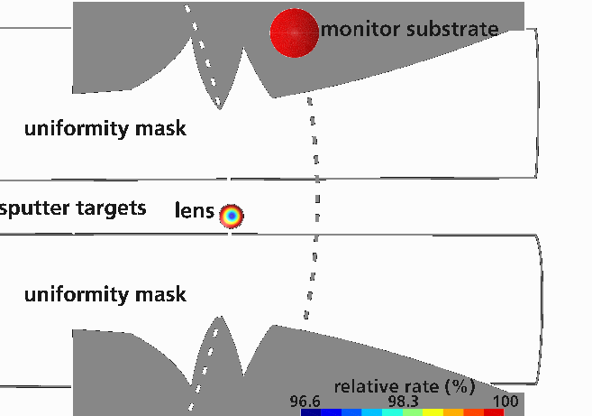
The geometry the optimisation works on: uniformity mask, sputter targets, lens and monitor substrate, with the resulting relative deposition rate. Source: Pflug, A. et al., Proc. 15th ISSP (2019).
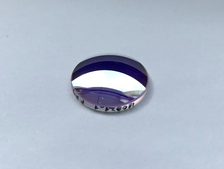
The result: the coated lens of the study.
Concave substrate for a membrane optics project
A rotating concave spherical substrate, argon plasma, silicon sputtering, a membrane at the target position. PICMC delivers the electron density in the plasma, the silicon flux towards the substrate and — as the actual result — the static absorption profile on the substrate. Profiles taken at different arm positions of the rotation agree with the measurement. The same run also produces the angular and energy histograms of the Ar⁺ ions and Si atoms that reach the membrane, which is the input for the atomistic growth simulation.
Macroparticles: where does the contamination come from
Dust in a PVD coater is a separate problem that reuses the same plasma results. PALADIN takes the DSMC / PIC-MC output as input and traces macroparticles through the gas, modelling what actually acts on them:
- charging and de-charging in the plasma,
- gas friction,
- thermophoresis,
- van der Waals forces at surfaces.
What comes out is not a single trajectory but statistics: a spatially resolved contamination profile, a size distribution, and the distribution of forces along the paths. The most useful output in practice is the backward question — which part of the target or of the chamber is likely to produce a particle that later reaches the substrate. In one case the answer was "particles generated close to the plasma", which identified them as target agglomerates and gave a starting point for countermeasures. Most of these particles do not even adhere to the substrate, but the impact alone can damage the coating.
Coupling to CFD
For processes where the gas flow is not in the free-molecular regime — atmospheric plasma, ventilated chambers, particle transport in air — the background flow comes from a CFD code (OpenFOAM, COMSOL) and only the particle and plasma part is done here. The same macroparticle code is used for aerosols in room air and for particles in liquids, which is how the method travels outside coating.
What the chain does not do
- Atomistic film growth is external. Columnar growth, density and stress of the growing film are simulated by a separate kMC/MD code (for example NASCAM). PICMC supplies the flux that goes into it.
- Optical design is external. The spectra that a layer stack produces are computed by an optical model; the chain delivers thickness and angle distributions for it.
- The chain needs calibration. Cross-sections, sputter yields and surface coefficients are only as good as the measurements behind them. A model that was never compared with a coated sample is a hypothesis, not a prediction.
What comes next
The case studies in the examples above are usually condensed into simple design rules — substrate thickness, pressure range, curvature limit, magnetic angle — because that is what a process engineer can use at the machine. The direction the framework is moving in:
- embedding the chain into recipe development as a routine tool rather than a project,
- surrogate models to make the parameter loops fast enough for large process windows,
- coupling with in-situ diagnostics so that the model is recalibrated during production.
Where to start with PICMC
If you want to use the PICMC stage of this chain:
- Parameter file for the setup, including the surface definitions that receive the ion flux.
- Averaged quantities for the time averaging that makes the flux usable by the next stage.
- Particle output for the files that leave a run.