Version: release 25

How to visualize electron movement in an existing plasma

Problem

The electron movement can be visualized via the 'POSITION' plots. In order to properly resolve the movement trajectory of typical electrons in magnetron plasma discharges, the time interval of the POSITION plot should be set to 0.1 ns.

The problem is that there are usually too many simulation particles and thus, the POSITION plots are difficult to visualize.

One possibility is to put only a few single electrons in an existing magnetic field configuration, however these electrons are not representative for electrons within a magnetron plasma discharge.

Solution

Use of adapted species and cross section file

The solution is to start from an existing plasma simulation and show only a small fraction of the electrons as "representatives". Additional "representative" electron species are to be created in the which are to be plotted in the POSITION plot. For that purpose, the file species_definition.r needs to be copied into the local folder and extended in the following way:

block GenSPEC : { float mr, charge, is_frozen = 0; };

Record SPECS = {
  Record e          = GenSPEC + { mr = 1/1823;   charge = -1.0; };
  Record eSec       = GenSPEC + { mr = 1/1823;   charge = -1.0; };
  Record eGas       = GenSPEC + { mr = 1/1823;   charge = -1.0; };

  ...

Here, the original electron species e is copied to the identical species eGas and eSec. The idea is to modify the gas phase reactions in a way that in a small percentage of ionizations, eGas is created instead of e. Analogously, the surface reactions are modified in a way that in a small percentage of cases, eSec are generated as secondary electrons instead of e.

Obviously, the cross section file sigma.r must be modified to include the additional species eGas and eSec which should behave the same way as regular electrons e:

...
  # ========================================================
  # Plasma interactions of electrons and argon [A.V. Phelps]
  # ========================================================
  block e_Ar -> {
    block list[] -> [
      CG.FCTeV_Entry + {
        MSG="$('e' %11s) + $('Ar' %11s) -> e + Ar (Elastic Momentum Transfer)";
        sigma-> (eV>0) ?   (abs(6/(1+(eV/0.1)+(eV/0.6)^2)^3.3-1.1*eV^1.4/(1+(eV/15)^1.2)/(1+(eV/5.5)^2.5+(eV/60)^4.1)^0.5)
                         + 0.05/(1+eV/10)^2 + 0.01*eV^3/(1+(eV/12)^6))*1.0E-20 ! MIN_SIGMA;
      },
      CG.FCTeV_Entry + {
        MSG="$('e' %11s) + $('Ar' %11s) -> e + Ar* (Total Excitation)";
        EV_THRESH = 11.5;
        flag_1 = 0; flag_2 = 1;
        if (defined(Properties.Arex)) then rp_vec = ["Arex"];
        sigma-> (eV>EV_THRESH) ?   0.85*(4E-22*(eV-11.5)^1.1*(1+(eV/15)^2.8)/(1+(eV/23)^5.5)
                                 + 2.7E-22*(eV-11.5)/(1+(eV/80))^1.9) ! MIN_SIGMA;
      },
      # Splitting: 5% probability of generating eGas
      CG.FCTeV_Entry + {
        MSG="$('e' %11s) + $('Ar' %11s) -> 2e + Arplus (Ionization)";
        EV_THRESH = 15.8;
        flag_1 = 0; flag_2 = 1;
        rp_vec = ["e", "Arplus"];
        sigma-> (eV>EV_THRESH) ? 0.98*(9.7E-18*(eV-15.8)/(70+eV)^2 + 6E-22*(eV-15.8)^2*exp(-eV/9)) ! MIN_SIGMA;
      },
      CG.FCTeV_Entry + {
        MSG="$('e' %11s) + $('Ar' %11s) -> e + eGas + Arplus (Ionization)";
        EV_THRESH = 15.8;
        flag_1 = 0; flag_2 = 1;
        rp_vec = ["eGas", "Arplus"];
        sigma-> (eV>EV_THRESH) ? 0.02*(9.7E-18*(eV-15.8)/(70+eV)^2 + 6E-22*(eV-15.8)^2*exp(-eV/9)) ! MIN_SIGMA;
      }
    ];
  };

  block eSec_Ar -> {
    block list[] -> [
      CG.FCTeV_Entry + {
        MSG="$('eSec' %11s) + $('Ar' %11s) -> eSec + Ar (Elastic Momentum Transfer)";
        sigma-> (eV>0) ?   (abs(6/(1+(eV/0.1)+(eV/0.6)^2)^3.3-1.1*eV^1.4/(1+(eV/15)^1.2)/(1+(eV/5.5)^2.5+(eV/60)^4.1)^0.5)
                         + 0.05/(1+eV/10)^2 + 0.01*eV^3/(1+(eV/12)^6))*1.0E-20 ! MIN_SIGMA;
      },
      CG.FCTeV_Entry + {
        MSG="$('eSec' %11s) + $('Ar' %11s) -> eSec + Ar* (Total Excitation)";
        EV_THRESH = 11.5;
        flag_1 = 0; flag_2 = 1;
        if (defined(Properties.Arex)) then rp_vec = ["Arex"];
        sigma-> (eV>EV_THRESH) ?   0.85*(4E-22*(eV-11.5)^1.1*(1+(eV/15)^2.8)/(1+(eV/23)^5.5)
                                 + 2.7E-22*(eV-11.5)/(1+(eV/80))^1.9) ! MIN_SIGMA;
      },
      CG.FCTeV_Entry + {
        MSG="$('eSec' %11s) + $('Ar' %11s) -> e + eSec + Arplus (Ionization)";
        EV_THRESH = 15.8;
        flag_1 = 0; flag_2 = 1;
        rp_vec = ["e", "Arplus"];
        sigma-> (eV>EV_THRESH) ? 9.7E-18*(eV-15.8)/(70+eV)^2 + 6E-22*(eV-15.8)^2*exp(-eV/9) ! MIN_SIGMA;
      }
    ];
  };

  block eGas_Ar -> {
    block list[] -> [
      CG.FCTeV_Entry + {
        MSG="$('eGas' %11s) + $('Ar' %11s) -> eGas + Ar (Elastic Momentum Transfer)";
        sigma-> (eV>0) ?   (abs(6/(1+(eV/0.1)+(eV/0.6)^2)^3.3-1.1*eV^1.4/(1+(eV/15)^1.2)/(1+(eV/5.5)^2.5+(eV/60)^4.1)^0.5)
                         + 0.05/(1+eV/10)^2 + 0.01*eV^3/(1+(eV/12)^6))*1.0E-20 ! MIN_SIGMA;
      },
      CG.FCTeV_Entry + {
        MSG="$('eGas' %11s) + $('Ar' %11s) -> eGas + Ar* (Total Excitation)";
        EV_THRESH = 11.5;
        flag_1 = 0; flag_2 = 1;
        if (defined(Properties.Arex)) then rp_vec = ["Arex"];
        sigma-> (eV>EV_THRESH) ?   0.85*(4E-22*(eV-11.5)^1.1*(1+(eV/15)^2.8)/(1+(eV/23)^5.5)
                                 + 2.7E-22*(eV-11.5)/(1+(eV/80))^1.9) ! MIN_SIGMA;
      },
      CG.FCTeV_Entry + {
        MSG="$('eGas' %11s) + $('Ar' %11s) -> e + eGas + Arplus (Ionization)";
        EV_THRESH = 15.8;
        flag_1 = 0; flag_2 = 1;
        rp_vec = ["e", "Arplus"];
        sigma-> (eV>EV_THRESH) ? 9.7E-18*(eV-15.8)/(70+eV)^2 + 6E-22*(eV-15.8)^2*exp(-eV/9) ! MIN_SIGMA;
      }
    ];
  };
  ...

In this modified my_sigma.r the reaction path between electrons and Argon are copied also for eGas and eSec, because the latter should behave the same way as regular electrons e. Additionally, in the reaction e_Ar the ionization is split into two reactions with 98% and 2% probability, respectively. In the first ionization reaction, regular electrons are created as reaction product, however the alternative ionization branch creates eGas particles.

Modified parameter file including creation of POSITION plots and representative secondary electrons

The modified parameter file shall produce POSITION plots in a high plot frequency and also include the production of "representative secondary electrons" eSec in the surface reactions.

To start from an existing simulation the following files should be copied into the folder of the new simulation case:

The whole checkpoint/* folder
The file last_shutdown.txt

The global variables of the PAR file should be modified to include the small plot interval of 0.1 ns:

# Parameter file for the PICMC gas discharge and DSCM gas flow simulation

# ===============================================
# Global variables
# ===============================================
DT       = 1e-11;    # Time step width
TSIM     = 2e-5;     # Total simulation time in seconds
TAVG     = 1;        # Time averaging mode (0 = off, 1 = on)
NPLOTS   = 200000;   # 0.1 ns interval
NDUMPS   = 1;        # Number of particle data dumps
WORKMODE = 1;        # Work mode (0 = DSCM gasflow simuation, 1 = PICMC plasma simulation, 2 = electric field solver)
T0       = 300;      # Initial particle and border temperature [K]
PSOLL    = 2;        # Aimed power dissipation in Watt (plasma simulation only)
PSAMPLE  = 1e-7;     # Sampling time for power dissipation (plasma simulation only)
VPMAX    = 700;      # Maximum voltage for power control (default = 1000 volt)

# ==============================================
# Specify species list
# Check SIM-Wiki for list of available species and reactions
# ==============================================
SPECIES  = ["Ar", "Arplus", "e", "eSec", "eGas"];     # List of species strings

NREAL_Ar     = 5e9;   # Default scale factor for Ar
P0_Ar        = 0.8;    #
SEY          = 0.12;   # Nb Secondary electron yield

# Comment/uncomment accordant to defined species:
NREAL_Arplus = 5e4;    # Default scale factor for Arplus
P0_Arplus    = 1e13;   # Default density of initial Arplus distribution [Number/m^3]

NREAL_e      = 5e4;    # Default scale factor for e
P0_e         = 1e13;   # Default density of initial e distribution [Number/m^3]

NREAL_eSec   = 5e4;    # Default scale factor for e
P0_eSec      = 0;   # Default density of initial e distribution [Number/m^3]
NREAL_eGas   = 5e4;    # Default scale factor for e
P0_eGas      = 0;   # Default density of initial e distribution [Number/m^3]
# ===============================================
# 3D data extraction
# Examples: NUMBER = ["Ar", "e"]; FIELD = ["PHI", "E"];
# ===============================================
NUMBER      = [];
DENSITY     = [];
PRESSURE    = [];
TEMPERATURE = [];
ENERGY      = [];
VELOCITY    = [];
ABSORPTION  = [];
# POSITION plots can get very large, so handle with care!
POSITION    = ["eSec", "eGas"];
# "PHI" = electric potential, "PHI_MEAN" = time averaged electric potential, "E" = electric field
FIELD       = [];

# For COVERAGE and DEPOSITION fill in required surface materials:
COVERAGE    = [];
DEPOSITION  = [];
...

First, there are 200000 plots for a physical time interval of 20 µs yielding a plot interval of 0.1 ns.

Second, the species list is extended by the representative species eGas and eSec. They get the same NREAL values as regular electrons and a starting density of zero (because they should be created by the gas and surface reactions in order to represent real electrons in the given plasma!).

In the plot section all regular plots are disabled and only the POSITION plots for eSec and eGas are enabled. This is important due to the high plot frequency - otherwise your harddisk space will be quickly flooded!

In the surface reactions, we have to add a branch with a low probability to create "representative" secondary electrons eSec:

  ...
  block Ar_Plasma_ext: {
    show_reaction_message("Simple Ar plasma-wall model (legacy version); SEY = $(PAR.SEY)");

    add_plain_reaction("Arplus", 1, 0.8, ["Ar", "e"], [1, PAR.SEY]);
    set_emission_energy("e", 0, 10, 100);
    add_absorption("e", 1.0);

    add_plain_reaction("Arplus", 1, 1, ["Ar", "eSec"], [1, PAR.SEY]);
    set_emission_energy("eSec", 0, 10, 100);
    add_absorption("eSec", 1.0);

    add_absorption("eGas", 1.0);
  };
  ...

This looks like a regular Ar plasma chemistry, where Arplus ions hitting the surface are neutralized and create secondary electrons. However the reaction branch for creating secondary electrons is doubled. In the first reactionm a reaction probability of 80% is given, while the second reaction branch has 100% probability¹.

Depending on the simulation case and electron density etc. it might be necessary to adapt the reaction branching probabilities in order to create the desired amount of "representative" electrons.

Example

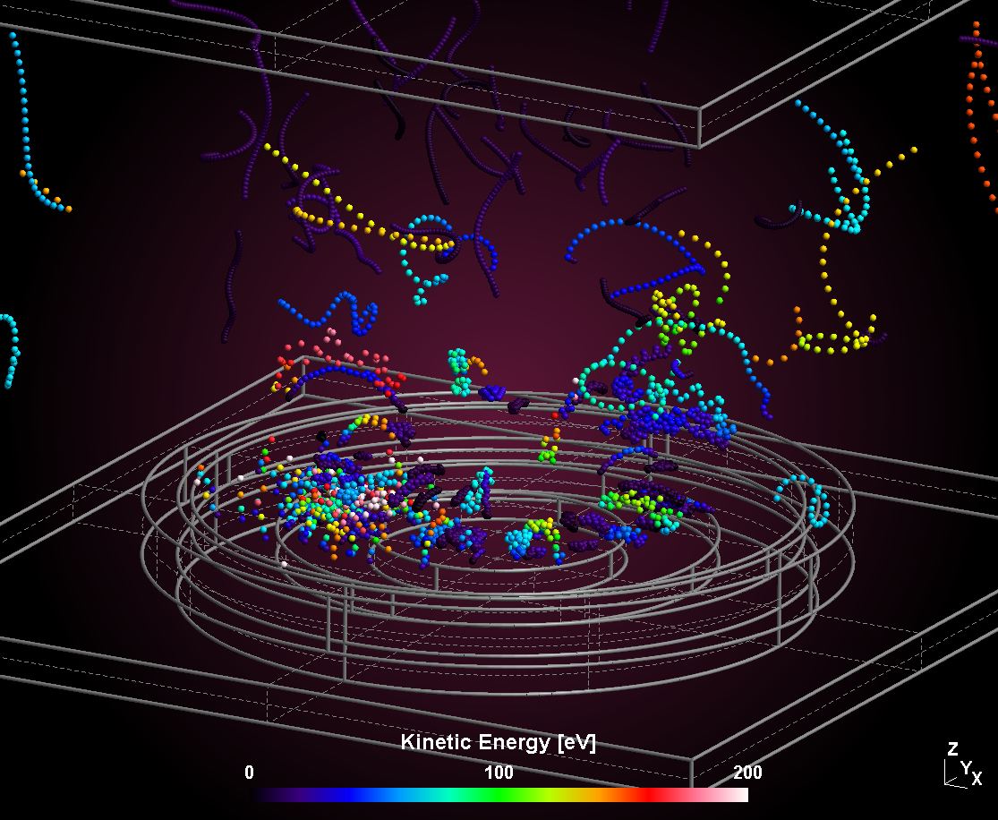
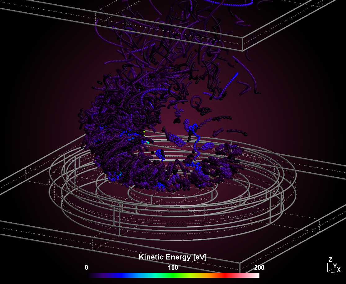
The example below shows trajectories of secondary electrons created at the target surface (left) and bulk electrons created by gas phase electrons (right). As can be seen, both groups of electrons differ strongly in their mean kinetic energy. Especially secondary electrons, which escape the magnetic confinement can gain the full target voltage as kinetic energy, while bulk electrons are equilibrated by numerous gas collisions and have some mean kinetic energy in the order of 5 eV.

The example is taken from a 3D model of a circular sputtering target. The trajectories are shown for a time interval of 10 ns with a plot interval of 0.1 ns (100 positions), respectively.

Secondary electrons	Gas electrons

Please note that multiple surface reactions are checked from top-down, i.e. if the first reaction is executed with 80% probability there is only 20% probability that the second reaction applies. Thus, the 80% - 100% probabilities are effectively translated to 80% - 20% reaction probability of both branches. This is unlike cross section lists, where multiple reaction entries are constantly shuffled during a simulation run in order to avoid such conditional probability issues. ↩

Problem​

Solution​

Use of adapted species and cross section file​

Modified parameter file including creation of POSITION plots and representative secondary electrons​

Example​

Footnotes​

Problem

Solution

Use of adapted species and cross section file

Modified parameter file including creation of POSITION plots and representative secondary electrons

Example

Footnotes