Fitting with SciPy
Basic idea and workflow
The raytracer can calculate the particle flux intensity reaching a substrate in a given scenario. In many cases this routine can be used for optimising coating processes by adjusting mask geometries or trajectories, for example.
This can be automated by using fitting routines. The algorithm is designed in a way that makes fitting relatively simple: a function has to be written that takes a vector of parameters, calls the raytracing routine and then calculates a number based on its output, which it then returns. Using the numerical optimisation methods provided by SciPy, the vector of parameters is iteratively adjusted to either minimise or maximise that number.
A simple example
scipy.optimize.least_squares minimises a given function. A minimal illustration:
# Import the least_squares routine from SciPy (make sure to have SciPy installed)
from scipy.optimize import least_squares

# Required for some methods in this example
import math

# Define a function that takes a parameter vector and returns a number
def fit_example(params):
  # Take the first value of the parameter vector
  x = params[0]

  # Some example function that has its minimum at x = 10
  return 1.0 - math.exp(-(x - 10)**2)

# Let's assume we don't know where the minimum is and guess the initial value 5 for x
# We also restrict x to the range between 0 and 20
final_result = least_squares(fit_example, [5], bounds = ([0], [20]))

# Print the result
print(final_result)
The result will look something like this:
     message: `gtol` termination condition is satisfied.
     success: True
      status: 1
         fun: [ 0.000e+00]
           x: [ 1.000e+01]
        cost: 0.0
         jac: [[ 1.490e-07]]
        grad: [ 0.000e+00]
  optimality: 0.0
 active_mask: [0]
        nfev: 2
        njev: 2
The important part is that x is 10, as expected. The approach extends to more than one variable
trivially, simply by extending the vectors.
The goal function
Any scenario becomes fittable by wrapping it in a function that returns a single number. Uniformity, as the helper module defines it: zero for a perfectly uniform coating, one for no coating at all.
def uniformity_of(s):
  values = s.dump_list(offset = SRT.PhysVector(0.0, 0.0, 0.0), normalize_to = 1.0)
  return sum((1.0 - patch[-1]) ** 2 for patch in values) / len(values)
SRTHelper.get_uniformity_of_substrate(s) computes the square root of that, and
SRTHelper.get_manhattan_uniformity_of_substrate(s) the linear version. Total and maximum intensity
are available as get_total_intensity_of_substrate(s) and get_max_intensity_of_substrate(s).
The linear version is the sum of the differences between 1 and the relative intensity of each patch, divided by the number of patches:
def uniformity(params):
  # ... (Do something with the params vector here)

  while not rt.finished():
    rt.step()

  intensity_list = s.dump_list(offset = SRT.PhysVector(0, 0, 0), normalize_to = 1.0)

  # Division by the number of patches is not strictly necessary, but normalises the
  # result to the range 0 ... 1, which helps the optimiser
  return (len(intensity_list) - sum([patch[-1] for patch in intensity_list])) / len(intensity_list)
Maximising the total intensity works the same way, by inverting the sum:
def maximum_intensity(params):
  # ... (Do something with the params vector here)

  while not rt.finished():
    rt.step()

  intensity_list = s.dump_list(offset = SRT.PhysVector(0, 0, 0), normalize_to = 0.0)

  return 1.0 / sum([patch[-1] for patch in intensity_list])
Any other target works the same way: a thickness profile that compensates the curvature of a lens, a ratio between centre and edge, a fit against a measured spectrum.
A comparison against a radial target profile is not built in — the helper that would do it is commented out in the source because it does not handle the substrate curvature yet. It is a few lines in the style above: loop over the radial patches, take the target value at that radius and sum the squared differences.
Reusing the raytracer
Inside the optimisation the raytracer is reset, not rebuilt. Creating a new instance per evaluation throws away the precomputed self-intersections and costs most of the run time for concave substrates.
def fit_function(params):
  s.reset_intensities()         # throw away the old intensities
  rt.reset_time_step()          # start the trajectory again
  m.reset_nodes_and_elements()  # empty the mask, keep its name

  # rebuild the mask from the parameters
  n0 = m.add_node(SRT.PhysVector(185.0, 170.0, 380.0))
  n1 = m.add_node(SRT.PhysVector(303.1, 184.9 + params[0] - 100.0, 380.0))  # free node
  m.add_circle_arc(n0, n1, -117.5)

  # mirrored masks have to be rebuilt as well
  rt.delete_mask(name = "UniformityMirror", has_to_exist = False)
  rt.mirror_mask(template_name = "Uniformity", new_name = "UniformityMirror",
                 mirror_point = SRT.PhysVector(-232.0, 260.0, 380.0),
                 mirror_axis = SRT.PhysVector(1.0, 0.0, 0.0))

  while not rt.finished():
    rt.step()

  return uniformity_of(s)
What can be reset and what cannot:
| Call | Effect |
|---|---|
s.reset_intensities() | All accumulated intensities back to zero |
rt.reset_time_step() | Time step back to 0, trajectory starts again |
s.generate_geometry(...) | New geometry and new ray intersections, intensities are kept |
m.reset_nodes_and_elements() | Mask contents emptied, name and thickness kept |
t.generate_...() / t.load_from_list(...) | Trajectory replaced |
rt.delete_mask(name, has_to_exist) | Mask removed; has_to_exist = False makes it a no-op if it is gone |
Mirrored masks keep their geometry when the template changes, so they have to be deleted and re-created. The same holds for their trajectory, which is not inherited.
Optimising the fitting process
Since the raytracing routine is called at every optimisation step, a few tricks are needed to get results with sufficient accuracy:
- No convergence guarantee. There is no guarantee that least squares converges, let alone onto the optimal parameter set. Evaluate a few sample values of the function first to get a feeling for where the optimum lies; the optimiser will then more reliably reach a local extremum.
- Bounds. Good bounds improve both stability and reliability. They also keep the geometry valid — see the next section.
- Tolerances.
xtol,ftolanddiff_steptrade speed against accuracy. This matters more here than in most fits: the default function tolerance of1e-8is far below the noise of an accumulated intensity field. - Cheap first pass. Limit the number of parameters, the number of substrate patches and the number of time steps. A simple planar substrate (disk or rectangle) already gives a rough estimate for the optimal trajectory or mask position, which can be refined afterwards with a detailed run.
Fitting mask geometries
General idea
A typical use case is to optimise a mask geometry in order to maximise the uniformity of a coating. Technically this can be done by using all mask node positions as free parameters, but that leads to long computation times and potentially invalid mask geometries, with connections crossing each other.
So do not go into this without a plan. Ideally you consider as few mask nodes as possible and keep the others fixed — mainly those with the largest impact on the uniformity.
Furthermore, proper bounds have to be passed for the node positions, because two connections of the mask must never cross. This can be checked on paper, as in the following figure.
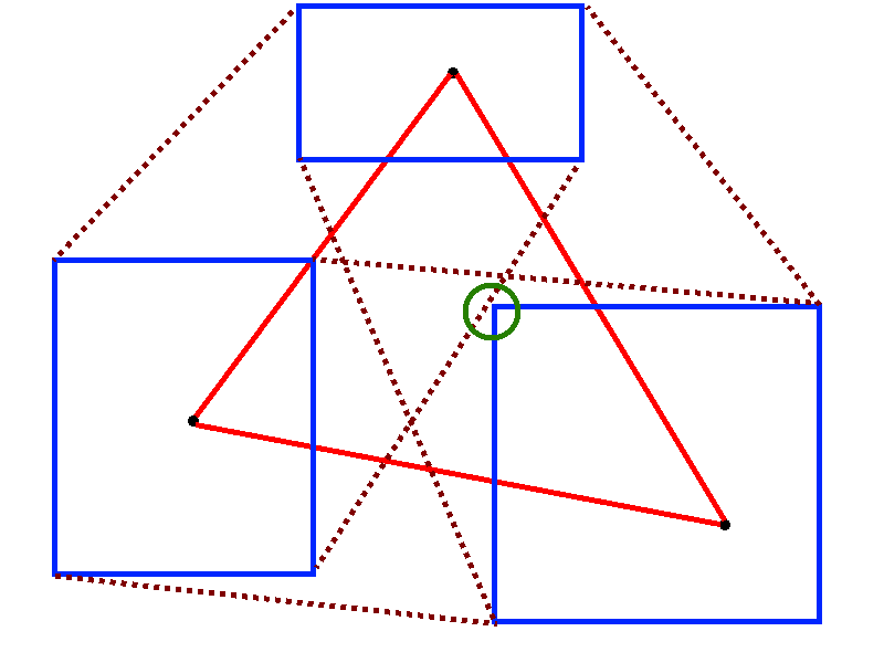
It is your job to prevent these situations by choosing appropriate bounds. Trial and error is a completely valid method, but drawing the mask and the bounds on paper also does the job.
Keep in mind that using low radius values for the connections can produce geometrically nonsensical connections, preventing the raytracer from working. Rather use high radii or straight lines for a first guess.
Python script
Please read the previous sections before simply copying this script. It optimises a rectangular mask for uniformity, based on a given histogram (which you need to provide); see Usage for the individual lines and the scenario.
import path.to.SRT as SRT
from scipy.optimize import least_squares

rt = SRT.Raytracer()
s = rt.get_substrate()
t = rt.get_trajectory()

# Substrate
substrate_geometry = "disk"
substrate_params = {
  "n_r": 10,
  "n_phi": 10,
  "radius": 100.0
}
s.generate_geometry(substrate_geometry, substrate_params)
if s.is_concave():
  rt.precompute_substrate_intersections()
s.set_sputter_up()

# Trajectory
traj_samples = 11
traj_radius = 540.0
traj_center = SRT.PhysVector(100.0, 100.0, 100.0)
traj_angle_start = -10
traj_angle_end = 10
traj_substrate_rotation = 90
t.generate_circle_arc(traj_samples, traj_radius, traj_angle_start, traj_angle_end,
                      traj_center, traj_substrate_rotation)

# Histogram
hist_batch = rt.add_histogram_batch("Test")
hist_filename = "histogram.txt"
hist_min_coords = SRT.PhysVector(0.0, 0.0, 100.0)
hist_max_coords = SRT.PhysVector(100.0, 100.0, 100.0)
hist_size_x = 20
hist_size_y = 10
hist_d_phi = 0
hist_swap_x_y = False
hist_batch.add_histogram_from_file(hist_filename, hist_min_coords, hist_max_coords,
                                   hist_size_x, hist_size_y, hist_d_phi, hist_swap_x_y)

# Mask
mask = rt.add_mask("Rectangle")
mask.set_thickness(1.0)

def my_function(parameters):
  s.reset_intensities()
  rt.reset_time_step()

  # Reset the contents of the mask
  mask.reset_nodes_and_elements()

  # Add all nodes and connections again
  node_0 = mask.add_node(SRT.PhysVector(parameters[0], parameters[1], 100.0))
  node_1 = mask.add_node(SRT.PhysVector(parameters[2], parameters[3], 100.0))
  node_2 = mask.add_node(SRT.PhysVector(parameters[4], parameters[5], 100.0))
  node_3 = mask.add_node(SRT.PhysVector(parameters[6], parameters[7], 100.0))

  # High values to model straight lines (until they're implemented properly)
  r_0_1 = 10000.0
  r_1_2 = 10000.0
  r_2_3 = 10000.0
  r_3_0 = 10000.0

  mask.add_circle_arc(node_0, node_1, r_0_1)
  mask.add_circle_arc(node_1, node_2, r_1_2)
  mask.add_circle_arc(node_2, node_3, r_2_3)
  mask.add_circle_arc(node_3, node_0, r_3_0)

  while not rt.finished():
    rt.step()

  intensity_list = s.dump_list(offset = SRT.PhysVector(0, 0, 0), normalize_to = 1.0)
  result = (len(intensity_list) - sum([patch[-1] for patch in intensity_list])) / len(intensity_list)

  # Give us some information about what's happening
  print(parameters, " -> ", result)

  return result

# Our starting values in pairs of xy-coordinates
fit_start_values = [100, 0, 0, 100, -100, 0, 0, -100]

# Minimum and maximum values, also in pairs of xy-coordinates
fit_min_values = [60, -40, -40, 60, -140, -40, -40, -140]
fit_max_values = [140, 40, 40, 140, -60, 40, 40, -60]

# Limit our required parameter accuracy to 1.0
parameter_tolerance = 1.0

# Limit our required function result accuracy to 0.001
function_tolerance = 0.001

# Only use steps of about 1% for the parameters
fit_steps = 0.01

# Start the fitting
final_result = least_squares(my_function, fit_start_values,
                             bounds = (fit_min_values, fit_max_values),
                             xtol = parameter_tolerance, ftol = function_tolerance,
                             diff_step = fit_steps)

# Print the final result
print(final_result)

# One more run with the optimum, for the output files
my_function(final_result.x)
What matters in practice:
- Few parameters. Every parameter costs a full raytracer run per iteration. Move one or two nodes, keep the rest fixed.
- Bounds, and a drawing. Every parameter box must be chosen so that no two connections of the mask can cross — a crossing mask produces nonsense, not an error.
- Tolerances. The default
ftolof SciPy is far below the noise of an accumulated intensity field.ftolaround1e-3andxtolaround0.1are realistic. - Cheap first pass. Fit on a flat disk with few patches and few time steps, then verify the result with the real geometry and a finer trajectory.
- Large value ranges. If one parameter is in millimetres and another one is a ratio, fit
normalised values in
[0, 1]and convert them back inside the function.
Questions
How can I apply tolerances to vastly different parameter values?
If you want to fit two parameters with entirely different value ranges, a single xtol or ftol
value for both is difficult to choose. In that case use normalised values as function parameters
(e.g. from 0 to 1) and calculate them back into their actual values inside the function.